
What is this?
This is my Software Engineering final year project for University from about 2003. I used to be work in the Fraud Detection industry (mortgage and credit card fraud) and this project was to solve a problem that I had found in the telecoms industry: fraudulent phone calls. It was impossible (for me) to get phone records from telecoms companies, so I had to build a tool that would model fraudulent calls and normal call patterns, I then had to build a tool that would detect calls that were fradulent from all of the call records.
The detector, iirc was a Multilayered perceptron Neural network, and it worked a little too well (which suggests my modelling was not adequaute.).
Anyway I learnt a lot.
Why are you posting this?
For fun mostly. I recently got linked to a project on Github that this project inspired, which then lead me down a hole that I had to follow, which lead me to finding my project and then I needed to post it.
https://github.com/mayconbordin/cdr-gen is the project that was based on my call detail record generator that was written in MS Access. :D
Enjoy the project!!
Note: Many of the TOC links don't seem to work :)
An Investigation into Real-time Fraud Detection in the Telecommunications Industry
Project Tutor
Dr Abir Hussain
Contents Page
7.2 Investigation into the Telecommunications Industry 14
7.2.1 Mobile Phone Telephony: 14
7.2.2 Fixed Line Telephony: 15
7.3. Investigation into Fraud 21
7.3.1 Who suffers from fraud? 21
7.4 Investigation of Fraud in the Telecommunication Industry 23
7.4.1 What is Telecommunication Fraud? 23
7.4.2 What does this mean to the Telecomm companies? 24
7.4.3 How is Fraud Perpetrated? 25
7.4.4 How do Telecomm Companies Respond to Fraud? 29
7.4.5 Some Key Attributes which may Identify Fraud. 30
7.5 Methods to Detect Fraud 31
7.5.1 Why Call Pattern Analysis is not always enough 41
7.6 Consideration of Real Time Methods 42
8 IDENTIFICATION OF PROBLEM AND SPECIFICATION 43
8.2 System Tools Research and Requirements 45
8.2.1 Further Requirements for the CDR Tool and Development Tool Research 46
8.2.2 Further Requirements for the Fraud Detection Prototype and Development Tool Research 49
9.3.1 Flow of Data When Creating a Model 62
9.3.2 Consideration of the UI 64
9.3.4 Data Representation and Considerations 64
9.3.4.1 Internal Data Representation 64
9.3.4.2 Customer Information 64
9.3.4.3 Entity Relationship 65
9.3.4.5 Index Considerations 67
9.3.4.6 Aggregating the Data 67
9.3.4.8 Testing the Model Generator. 69
9.5.1 What is a neural network? 72
9.5.2 Types of Neural Networks 76
9.5.3 What Neural network to use? 78
9.5.4 Training a Neural Network. 79
9.5.5 Training Method for the Feed forward Network 83
9.5.6 Problems Which can be Encounter when Training 84
9.5.7 Inputs defined in the NN. 85
9.5.9 Consideration of the Data Being Presented to the Network 89
9.5.10 Consideration of the Output of the Network. 90
9.6 Neural Network Creation Tools Design 92
9.6.3 Performance Analysis and Testing 95
9.6.4 Establishing the Most Appropriate Threshold for the Final Network. 101
9.6.4 Testing the Network Creation Tool. 102
9.7.1 Methods to generate the best models. 103
9.7.2 Brief discussion about the models used. 104
10.1 Overview of how to study the graphs 107
10.8.1 The weights from the input layer to the hidden node 122
10.8.2 The weights to the Output Layer 122
10.8.4 Proposed Training Regime 122
11.3 Which Training Method was Most Appropriate 125
11.4 Other Points About the Neural Network 125
13.1 How I handled the project 127
16.2.1.1 How to read the performance information off the CD 141
16.2.1.2 Function Descriptions 142
16.3 CDR Generation Tool Screen Shots 146
16.4.2 Neural Network Tools 152
16.6.2 Time Plan (Interim) 160
16.7 Interim Report & Specification 162
1. Abstract
An investigation into fraud detection in the telecom industry with a focus on development of a tool to help aid the detection process.
Neural networks were employed to find anomalous call patterns for customers over two week periods which matched call patterns of previously known fraud.
Customer information was generated using a bespoke tool and a final neural network was produced after rigorous testing which can successfully classify fraudulent and non fraudulent activity of customers.
Keywords: Fraud Detection, Software Engineering, Customer Detail Record, Database, Neural Network
2. Acknowledgements
I have enjoyed working on this project and I would like to thank my parents and family for the help and support that they have given me throughout this year.
I would also like to take this opportunity to thank Dr Abir Hussain for the help and support that she has given me as a project tutor this year.
I hope this report shows the amount of work and effort that went into this project during my final year studies.
3. List of FiguresFigure 1 Process of a customer of a telecomm company 18
Figure 2 The Fraud Management Cycle 29
Figure 3 Roles where an FMS Tool maybe used 32
Figure 4 Subscription Fraud 33
Figure 6 A) Non-linear problem separation B) Added Dimensions 39
Figure 7 Normal Linear Sequential Model (Waterfall) 43
Figure 8 Amended Linear Sequential Model (Waterfall) 43
Figure 9 Standard model for database communication 47
Figure 10 An Ideal situation for CDR Tool and Fraud Detection Tool 49
Figure 11 Processing the data through a neural network 49
Figure 12 Abstract overview of data flow in the system 53
Figure 13 A Gaussian distribution based on male heights in the UK 55
Figure 14 The Gaussian distribution function 56
Figure 15 Gaussian Distribution A 57
Figure 16 Gaussian Distribution B 57
Figure 18 Customer Generate tool flow diagram 63
Figure 19 Basic Entity Relationship for customer information 65
Figure 20 Overview of tables, fields and relevant joins used in the final output query 67
Figure 21 Sliding Window Effect 68
Figure 23 An artificial neuron based on Binary Threshold Logic Unit 73
Figure 24 Logistic Sigmoid function & Tan Sigmoid function 74
Figure 25 An artificial neuron based on a continuous sigmoid output function 74
Figure 26 Combining logsig(5x-2) + logsig(x+2) – logsig(2½x -12 ) 75
Figure 27 The Feed forward Neural Network 76
Figure 28 A Recurrent Network 77
Figure 29 Single Threshold system 90
Figure 30 Dual Threshold System 91
Figure 31 Training Tool Data Flow 94
Figure 32 Data extraction tool data flow 95
Figure 33 Y-Axis for ROC Chart (Sensitivity) 97
Figure 34 X-Axis for ROC Chart (1 - Specifity) 97
Figure 35 An incorrectly trained neural network ROC depiction 98
Figure 36 Actual output of an incorrectly trained network 99
Figure 37 ROC Chart for a working neural network 99
Figure 38 Data flow for establish the performance of the neural networks 101
Figure 39 Performance of the training algorithm 107
Figure 40 Output of the neural network after the test stage 108
Figure 41 Output of the neural network after the validation stage 109
Figure 43 MATLAB depiction of a 2 Layer network with 5 nodes in the hidden layer 112
Figure 44 MATLAB depiction of a 2 Layer network with 6 nodes in the hidden layer 113
Figure 45 MATLAB depiction of a 2 Layer network with 7 nodes in the hidden layer 114
Figure 46 MATLAB depiction of a 2 Layer network with 8 nodes in the hidden layer 115
Figure 47 MATLAB depiction of a 2 Layer network with 9 nodes in the hidden layer 116
Figure 48 MATLAB depiction of a 2 Layer network with 10 nodes in the hidden layer 118
Figure 49 ROC Chart for the best performing network 119
Figure 50 Output from the training data. 120
Figure 51 Performance of the final network while training 120
Figure 52 Output from the validation data 121
4. Glossary of Terms
|
4m's |
The four ms by FMS |
|
Bad Debt |
Unpaid Credit. Up until a while ago fraud was written of as bad debt, however they are fundamentally different |
|
BP |
Back propagation, used in the training of a feed forward neural network |
|
Cell |
A receiver or transmitter which a GSM phone communicates with |
|
False Negative |
Incorrect classification of an event considered to be TRUE; the event is given as FALSE |
|
False Positive |
Incorrect classification of an event considered to be FALSE; the event is given as TRUE |
|
FML |
A Fraud Management Company |
|
FMS |
Fraud Management System (A system used to detect and manage fraud) |
|
GSM |
Groupe Speciale Mobile, also known as Global Systems for Mobile Communication |
|
Internal Fraud |
Someone in the company is using inside knowledge to defraud the company |
|
IP |
Internet Protocol |
|
Means |
The nature of the fraud used to satisfy the motive |
|
Method |
The detailed method used in 4m's classification |
|
MLP |
Multi-layer Perceptron |
|
Mode |
The generic fraud method used |
|
Motive |
The objective of the fraud |
|
NN |
Neural Network |
|
NRF |
Non-Revenue fraud. Intent to avoid the cost of a call, but no intention to make a profit from it |
|
PABX |
Private Branch Exchange |
|
PRS |
Premium rate service |
|
True Negative |
Correct classification of an event considered to be FALSE; the event is given as FALSE |
|
True Positive |
Correct classification of an event considered to be TRUE; the event is given as TRUE |
|
UMTS |
Universal Mobile Telecommunications Service |
5. Introduction
The project aims to detect fraud in the telecommunication industry from the perspective of the customer and the telephone calls that they make. Several different method of detection can be used, but I intend to present one method that I feel is the most suitable for reasons given later in this project. At the end a prototype system will be presented to prove that the chosen method of fraud detection is feasible.
This project differs from the normal software engineering process, where the stakeholders would be identified. Requirements gathered from the stakeholders, with research into the system then taking place and the design processes following from this.
Rather it is an investigation into the how fraud occurs in the telecommunication industry and how it can be combated, with the added slant of a prototype system being implemented to show that a particular method can be used successfully to detect fraud.
Essentially I have identified a problem in the telecommunication industry, and after researching the problem area, I will propose a system that could be developed and produce a prototype of a system to show if it will work or not. It is not a case of building one prototype however, due to the nature of the prototype many will have to be created and empirically tested to find which prototype is the best performing .
This type of software engineering process, might be used for instance with a start up company or new business venture. They have found a market niche and they think they can exploit it by solving the problem. What is then required is a system of research and prototype development, if the prototype is not successful then it maybe that their current theory is not valid and a new direction of attack is needed.
The next chapter will include a brief introduction to the risk involved in this project and a summary of the research that I have done to make this project possible.
6. Risk
Often software engineers talk about inherent risk in each of the projects they undertake. This project is no different, even though the slant of this project is slightly different to what would be considered a "normal" software engineering project.
Pressman highlights eleven key components in overall risk for a project; however only a few can be uniquely attributed to this project 1 :
- Is the project scope stable?
8. Are the requirements stable?
10. Are there enough people on the team to complete the task?
As can be seen each of these key risks are associated with man-power and time taken to complete the tasks. If the project requirements are not stable, then the likelihood of a successfully completed project is minimised, since it is obvious that the requirements gathering process will be failing, thus indicating that the customer will not get the product they wanted. In relation to
Additionally, if the project has varying scope it means that the project will not satisfy the requirements which it was originally intended to.
The two highlighted risks can also have an adverse effect on the number of people needed to complete the task. The longer it takes to tack down a suitable product with stable requirements and a well defined project scope, then the more people the software development team are going to need to be able to successfully complete the project.
7. Research
7.1 Chapter Summary
In this chapter, various methods to detect telecommunication fraud will be investigated. This meant that I had to understand the telecoms industry. From this, I discovered that the telecoms industry is massive, with many different sectors; therefore a tool to detect general fraud is impractical for a project. This led me to focus on a subset of the industry. Further researching into this sub-sector, I found again that there are many different fraud types and methods to detect such fraud. Therefore I decided to further refine the category of fraud I was looking for.
Once I had decided on the type of fraud I would detect, it was important to understand the methods used to detect the fraud. It became known that the most suitable solution for me is to create a Neural Network based solution for reasons established in the following section.
7.2 Investigation into the Telecommunications Industry
The telecommunication sector is a huge arena. Each area of the sector covers a vast domain of communication. Identified below are several areas in which the telecommunication companies operate. These are mobile phone telephony, traditional land based communication, data transfer and the Next Generation mobile services.
7.2.1 Mobile Phone Telephony:
The phone system that is in use throughout Europe and the majority of the world is a standard called GSM (Global Systems for Mobile Communications). Each mobile phone registers itself to a "cell" (hence cellular phone) with which it can communicate by broadcasting over the airwaves to it's cellular base station, which will then essentially form a traditional circuit switched network with the destination 2 .
Traditionally cellular services offered have been more expensive than fixed line services, but are of similar nature and hence when setting up customer accounts services similar processes are adhered to; and accounts have to be paid for in a similar way. i.e. via a contract in which payment is required at the end of each billing period. Normally the contract would include a free phone as part of the deal.
However, more recently prepaid credit schemes are being used where the customers pay "up front" for the services they require and this includes having to buy the mobile phone. Prepaid credit was introduced into Europe in early 1996 3 as a method for the telephone operators to reduce the risk of having "bad credit" users on their system (people how have failed credit checks due to issues such as late bill payment). The system follows the same principle as the prepaid card schemes that have been used on public telephone systems for many years. The user buys a certain amount of "talk time" minutes from a retailer and inputs this into their mobile phone. The telecomm company is then aware of the credit available to that customer. Once the customer has used up all there credit, the phone will become unable to make out going calls (expect for emergencies and credit top up). This has been extremely popular with the teenage market, where contracts for mobile are not possible.
7.2.2 Fixed Line Telephony:
The traditional bread bearer of the telecommunication industry, with nearly every house (95% for 1999-2000) in the UK 4 having one or more telephone lines. Over these, normal voice traffic occurs, but in the last 10 years substantial increases in Internet Traffic, as many households get wired on to the Internet and drastic increases in daily use of the Internet (October 2002 reported that 45% of households have access to the Internet) 5 , have forced the telecommunication operators to reconsider the pricing structures they offer for their customers.
The services of a fixed line system are normally contract based, with the bill being settled by the customer at the end of each billing period.
Traditional operation of fixed line telephony is based on circuit switched networks. Which when a call is started, the local switch at the telecommunication substation makes a circuit (possibly via other switching stations) with the remote switch, which in turn rings the dialled telephone number. This circuit is then maintained for the duration of the call, and all information follows one fixed path to the destination 6 .
7.2.3 Data Transfer:
Initially data transfer services consisted solely of a carrier such as BT, providing a permanent connection to the Internet or between a companies' network. Essentially a dedicated communication line is being placed between both of the ends. Heavy contracts between the provider and the customer are drawn up and depending on the contract, in which payment terms can consider the quantity of data transferred as well as the speed of the line and what it is being used for 7 . It must be noted that BT normally provide the communication infrastructure, with other companies acting as partners reselling the service. This was initially put in place to stop BT becoming a monopoly 8 . These services where expensive, and designed mainly for the corporate sector. Because of leased line pricing structures and the work which needs to be carried out to connect customers to BT networks, leased lines were never meant to be available to the general public.
Other data transfer technologies exist and are coming to the forefront; ADSL (Asymmetric Digital Subscriber Line) and DSL (Digital Subscriber Line) are designed to operate over normal twister pair copper cable and thus are potentially available to every home in the UK. With the recent introduction of broadband Internet access services such as ADSL and DSL, providers have had to put in place extra facilities to handle the increased traffic, as they are responsible for the routing of the data on to the Internet.
7.2.4 Next Generation:
This is where the distinction of services differs from tradition mobile and fixed line services. Next Generation services more commonly known 3G are systems offering services such as video conferencing, video on demand, broadband Internet access across the air waves and are just some of the facilities that telecommunication companies are gearing up to accommodate.
The technology that 3G communication operates on is similar in nature to the method of current GSM, in the sense that each handset communicates with the base station in its cell; however, it uses a new communication protocol called UMTS (Universal Mobile Telecommunication Service). UMTS communicates on different frequencies and in a slightly different method to GSM, which allows vastly supplier data transfer rates 9 with the added advantage of allowing the mobile telecom companies a smooth transition between technologies.
Unfortunately for the telecom companies they invested a lot (£billions) of money in to acquiring the licenses for the use of the frequencies required by UMTS, so take-up by consumers may be slow as the telecomm companies may want to recoup some of their cost by heavily charging early adopters for use of the services. 10
Each of the above areas, have very similar sub-sections that when combined provide the final service to the customer (with the exception of data transfer services).
- Subscription: This is the initial contact that the telecommunication operator has with the customer. They will establish and verify the details of the customer. Once completed, the company will move on to the next stage of the process. This process will only happen once per client.
- Activation: Once the customer’s credentials have been verified and the subscription process has been completed, the customer will be set up on the network. This process may involve an engineer being used to create a connection at the user’s premises, or in the case of a mobile phone, the SIM card being activated. Like the previous stage (subscription), this should only occur once for the customer.
- Customer Use: The customer has been set up on the company’s network, and will be allowed to use the service with in the limits of the agreed parameters, such as credit limits and usage agreements. This will be established at the start of the contract, but will run throughout the lifetime of the agreement and depend on the any renegotiations of the contract.
- Billing & Payment: Coinciding with the “Customer Use” is the Billing of the service provided along with the payment, this could be seen as two separate sections, as they require both parties cooperation. The company will invoice the customer for the use of the network at set intervals (monthly, quarterly etc) outlined in their agreement. The customer is then expected (required) to pay for the services that they used in a timely manner set out in their contract.
Figure 1 Process of a customer of a telecomm company
- Termination of service: Once the contract has either been revoked by the operator or ceased at the request of the customer. The telecommunication company must issue a final invoice and then terminate the user's privileges for the system.
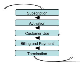
The previous processes (figure 1) will only occur once per account item, such that if the user request a new line or additional services, then the above steps will be repeated and will generally pursue the same structure.
Two important very important areas are in the previous process (figure 1); customer use, and billing. Whenever the customer uses their phone, information about the call parameters is logged; using this information the customers bills are calculated. Information is normally logged in what is called a CDR (Customer Detail Record or Call Detail Record, both of which can be used interchangeably) is as follows:
- Customer Number or ID
- Destination Number
- Call Type (PRS, International, Local etc)
- Call Start time
- Call time type (off-peak, on-peak)
- Call End time
- Duration and final cost of the call
The secondary bullet points are by-products of the parent point and are also sometimes a culmination of other points. For instance the final cost of the call, is a combination of call type, time of call and duration of the call. These by-products maybe generated at the time of the call so to speed up generation phone bill when it comes to the end of the customer billing period, or it might be generated when the bill is being worked out. The later requiring less storage space in the companies calls logs.
Other telecomm companies are another major source of revenue for a telecom company, they use a process called "Interconnection Charging". The telecom company will charge each of the operators for every call originating on the competitors network that is being routed to their network. For instance, BT will charge NTL a set fee for each call originating on NTL with a destination on BT. This practice is very common between mobile phone operators, as well as fixed lines operators 11 .
Now that the levels of service that the companies offer has been established, it is important to decide which areas that this project will concentrate on; this is because of the differences in the core services. An example, ADSL broadband accounts will not operate in the same way as mobile telephone accounts operate, thus the business processes and the implementation will be very different.
This project will focus on detecting fraud that can occur with circuit switched based communication methods, particularly call based systems not derived using IP solutions. In the next sections, topics will be covered with the emphasis on Fraud occurring in the following sectors:
- Mobile;
- Fixed Line,
Bearing the above market sectors in mind it must be noted that when detecting fraud for both sectors, only attributes that are present in both sectors can be used as indicators of fraud.
Common attributes of both Mobile and Fixed Line telephony in particular are the types of calls that take place. A mobile user will make calls to other mobiles, fixed lines (local and national), international numbers, free rate numbers, Premium Rate Service number (PRS). The same can be applied to users of fixed line services.
However when considering items that are dissimilar in both the technologies, issues such as when a mobile user makes a call, the current cell that it is in is also recorded. Obviously this is of no use when analysing call data for fixed lines.
7.3. Investigation into Fraud
Fraud on its own can be defined as "an intentional deception resulting in injury to another person" or "a person who makes deceitful pretences". Some useful synonyms can also be used do describe fraud [con, swindle, racket, hoax, scam, deceit, deception] and what a fraudster is [impostor, pretender, fake, faker, role player].
Fraud in general is a very broad subject, but can normally be boiled down to one easy description; "The need to make money". Fraud can be committed in many ways, for many reasons other than just "The need to make money" making many different people from all lifestyles, susceptible to fraud. Other reasons include crackers wanting kudos from their peers (breaking in to a system and taking information or money); people wanting to save money rather than make money, the list continues.
7.3.1 Who suffers from fraud?
In the end we all do, for instance: Fraud in the insurance industry due to false claims, can increase every customers premiums; Fraud in the financial industry, can mean higher rates of interest on things such as mortgages, loans and credit cards while also reducing the interest rates for savers; Fraud in the telecommunication industry can result in higher call bills. All because the companies that are being defrauded, still need to make money, so any loses due to fraud are normally passed on to the consumer.
Fraud against the individual is also another topic that needs a brief discussion. Fraud against the individual can take many different guises: A street seller may "persuade" a person into donating money to a dying child; A phone scammer may persuade people to part with their credit card details for a fictional product; or an email may dupe people into depositing money into a Nigerian bank account with a promise of returns far greater than those given.
The physiological effect of fraud as well is unmeasured but considerable. It is easy to see that if an individual (rather than a corporation) has been defrauded, a once normally confident person can easily be transformed into a person who no longer trusts his or her own judgement. Other than the financial difficulties induced, the fear of criticism from peers is also high, since perhaps the subject had to request to borrow money from a family member or business colleague. The increased fear of the parties finding out may result in anxiety, guilt, and fear of being held responsible. Possibly culminating in depression. 12
For both types of fraud (Fraud against a corporate and fraud against and individual) the number of different styles of fraud is uncountable. When the companies or law enforcement agencies think they have the hatch battened down on fraud, another scheme for the fraudsters presents itself and the cycle continues.
7.3.2 Who commits fraud?
Now that we have established a reason why fraud is committed, we must also ask what type of person commits fraud.
The type of people that commit fraud can be broken down into at least two categories:
The Opportunists; The opportunist commits fraud as a one off. Word of mouth may spread that a particular company is susceptible to fraud using a certain process . For instance, obtaining a loan by using false details. Or faking an injury to obtain more financial aid from an insurance company. The frauds in this case are normally committed by normal people who essentially want to gain a quick buck.
The Crime syndicate; The crime syndicate will normally commit fraud, to provide money for other crimes such as drug trafficking. They will hit a service for all the money that they can get. The people who operate theses systems, unlike the opportunist are very professional and will always be looking for new methods to defraud people and companies, since it is in their interest to keep providing extra money to the syndicate.
Fraud is unstoppable, even when an avenue to fraud has been closed, another will present itself; and as the fraud detection systems get more complex, the methods used to defraud people will also become more complex.
7.4 Investigation of Fraud in the Telecommunication Industry
When establishing what "Fraud" is in the Telecommunication Industry it is important to understand several questions.
- What is Telecommunication Fraud?
- What does Fraud mean to the Telecomm companies?
- How is the Fraud perpetrated?
- How do Telecomm companies respond to fraud?
- Some key attributes which may identify fraud.
7.4.1 What is Telecommunication Fraud?
The Telecommunications (Fraud) Act 1997 highlights effectively what Fraud is in the Telecommunication industry. In broad terms the act states, "To use or obtain a service dishonestly" and including "To use or to allow the supply of a dishonest service" is considered to be fraud. 13
Fraud in the telecommunication industry can be broken up into two major sections. The first being revenue based fraud, and the second being non-revenue based fraud.
Revenue fraud consists of any type of fraud with the purpose to make the individual who is perpetrating the fraud, money. This can be achieved in such ways as:
- Selling high cost International calls to people by severely undercutting the cost that the telephone company charges;
- Calling high rate PRS lines, with no intention to pay for the cost of the call.
Non-revenue fraud is normally fraudulent use of the telecommunication network for reasons other than making money. Motivations for non-revenue fraud include:
- Removing any chance of criminals being surveyed or having phones tapped, by criminal investigation agencies by making illicit use of the network;
- To provide free or heavily reduced call costs to friends and family;
- To show to their peers (other crackers) that they do have the skill to breach the telecomm companies' security.
7.4.2 What does this mean to the Telecomm companies?
It has been reported that worldwide that fraud accounts for approximately 3% 14 of the Telecomm companies' annual revenue. In 1999 the UK alone suffered losses of at least £720 Millions split over the following categories. 15
|
Calling Card |
Cellular |
International |
Other |
Total |
|
$150 Millions |
$100 Millions |
$500 Millions |
$250 Millions |
$1100 Millions |
Table 1 Losses Due to Fraud in the UK (in dollars)
However, this only accounts for fraud that has been detected, since fraud can often go undetected and unreported. Fraud may go unreported or at least unpublished due to the nature of business contracts and customer confidence if the perceived levels of fraud are high in relation to the revenue generated. The knock on effects of fraud and lost income include higher bills as the losses are passed on to the customer, and higher churn rates for the company when more people are unsatisfied with the service and the perceived security that the company offer. Add this all together and it can negatively effect share holders confidence as annual revenue is decreased and expansion is drawn back.
7.4.3 How is Fraud Perpetrated?
Telecomm Fraud can be broken into several generic classes. These classes describe the mode in which the operator was defrauded and include subscription fraud, call surfing, ghosting, accounting fraud and information abuse 16 . Each mode can be used to defraud the network for revenue based purposes or non-revenue based purposes.
7.4.3.1 Subscription Fraud
Subscription fraud occurs when an unsuspecting party have their identity stolen or a customer tries to evade payment. Essentially, personal details provided to the company are erroneous and designed to deceive the company into setting up an account. Reasons for this may include a customer knowing that they are a credit liability due to CCJ's or other credit problems; or a fraudster needs to obtain "legitimate" access to the telecomm network to perpetrate further modes of fraud.
Subscription fraud causes serious financial loses to the telecommunication operators, but in many instances may not be attributed to fraud. If someone does not pay their bill, then the telecomm company has to establish if the person was fraudulent or is merely unable to pay. This may result in a lot of subscription fraud being classified as bad debt. The BT Group in 2001-2002 estimated that bad debt cost the company ~£79 million. 16
7.4.3.2 Call Surfing
Call Surfing is when an outside party will gain unauthorised access to the operators network through several methods such as call forwarding, cloning, shoulder surfing.
Call Surfing can include gaining access to a company's PABX (Private Branch Exchange) either via social engineering, or by lack of security. Social Engineering could be considered as: A person rings the company's telephone administrators claiming to be a BT engineer performing a line test, they ask for the password so that they can negotiate access to the call-back of the PABX; or a employee in a large company receives a call from a person claiming to have got the wrong extension, and requests if they could put them through to extension 901, with 9 being the external dialling code of the PBX and 01 being the international prefix. 18
These may be unrealistic scenarios, but it is all too easy for someone to gain access to a system this way. Once the cracker has access to the PABX, they can use it to forward calls internationally or to premium rate service lines. All they pay for is the cost of the call to the company, while the company picks up the cost call to the proper destination. The cracker may even escape paying for the original call if they covered their tracks, for instance via subscription fraud.
Cloning of mobile phones is another issue that will arise, especially since the early mobile phones operated on analogue with the signal emanating from the phone being easy to detect and read, and thus the technology used to identify each phone uniquely was susceptible to being read. With this information, the fraudster would be able to reprogram one of their own phones to match these unique details. Once done, the con artist would be able to use the phone to make all the calls that they needed without the original phone owner knowing (until they get the telephone bill that is). 19
7.4.3.3 Accounting Fraud
Accounting Fraud can occur through manipulation of accounting systems and maybe used to help someone avoid having to pay for the service. Normally this is an internal problem. Accounting Fraud would normally occur, when someone would want to try and get cash back at the end of their billing period, or have their bill reduced. 20
7.4.3.4 Ghosting
Ghosting requires knowledge of the internal systems, maybe an employee would set up an account that would not need to be billed or remove billing details from the system. On the other hand, schemes may involve creating a piece of tone generating hardware that will fool the switch centre into thinking that a call might be a free call, or is operating from a public telephone. Essentially, they are "Ghosts" on the system as there is little or no trace of them ever being present on the network. 21
7.4.3.5 Information Abuse
Information Abuse occurs when an employee can use the telecommunications companies software to access privileged information about clients or systems. This information maybe passed on to third parties and used in further fraud. However, it is not solely limited to this, for instance company A might place spies into company B to find out information about any alliances that company B might have. Again, this is an internal fraud. 22
FML (A Fraud management company) developed a system called the 4m's to help fraud analysts decide if a particular case they are studying is more than likely fraudulent. It can be used to understand where each of the previously (section s 7.4.3.1 – 7.4.3.5) mentioned methods to perpetrate fraud and the reasons for doing so fit in with each case of fraud. 23
The 4m's can be defined as Motive, Mean, Mode and Method:
- Motive: This is the reason why they will commit the fraud. This could range from generating money, saving money, kudos or just malicious intent.
- Mean: Used to satisfy the motive. If it is revenue based fraud, how are they getting their money: by selling International calls at a reduced rate; calling PRS services; using access codes supplied by an informant.
- Mode: This is the generic method used to commit the fraud. Such as subscription fraud or call surfing.
- Method: This is the way in which the fraud was committed. For instance, how the call surfing was achieved.
An example of where this system of classification could be used: A person orders a new telephone line with incorrect identification details, once the telephone line has been installed; the person offers International and PRS calls at heavily reduced rates. Then after the billing period the person vanishes and never uses the phone again.
Fitting the above example into the 4m's classification we can see that the persons Motive was to make money. Their Means was via Call Selling. The Mode was using vulnerability in the telecom companies subscription process (Subscription Fraud) and the Method was using False details with no intent to pay for the services used.
A second example of where this classification could be used is: An employee who works in the calling card printing division sells valid pin numbers for pre-paid calling cards to third parties.
Applying the 4m's classification, we can see that their Motive would be to make money. Their Mean is Facilitation to supply fraudulent access to the network. The Mode is via Information Abuse and the Method was disclosure of pre-paid card number.
7.4.4 How do Telecomm Companies Respond to Fraud?
Telecommunication companies will respond to cases of frauds in a manner that is similar to those used in the financial industry.
The telecommunication operator should have a company wide fraud management scheme, which can be broken down into four discrete steps (figure 2) 24 .
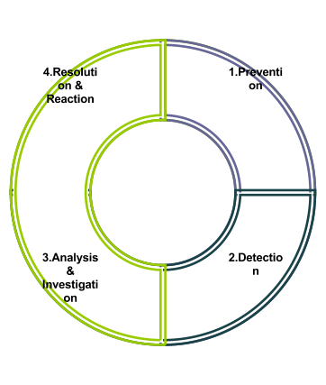
- Prevention
- Detection
- Analysis & Investigation
- Resolution & Reaction
Prevention is the most important, if the fraud is stopped before it happens, the less money a company will lose.
Figure 2 The Fraud Management Cycle
However, if it cannot be prevented the next best thing that the can happen is to detect it either when it happens or in the early stages of it occurring. This will mean that losses will be reduced from what they would have been if the fraud had gone undetected.
Once a case has been detected, analysis must take place to ensure that a customer account is being abused, since if service is withdrawn for insufficient reasons, customers maybe entitled to pursue legal action against the company.
Once sufficient motive has been established, it is then up to the company how they choose to react. For instance disabling the account and placing measures to prevent (stage 1) the type of fraud from reappearing, is the ideal solution.
Unfortunately, the measures taken are normally reactionary, since the fraud has already occurred. The company will receive an indication that a customer account is potentially fraudulent. It is up to the company to investigate the claim. Only then once enough evidence has been established that fraud was taking place with the customer can the telecommunication company can take appropriate action to remove the fraud from the network
7.4.5 Some Key Attributes which may Identify Fraud.
A telecommunication company will look for several key attributes when trying to ascertain if a fraudster is trying to use their network 25 :
- The customer is new to the network, and has requested many features of the phone system straight away.
- The customer has high average call duration and high average calls cost, can indicate PRS or International fraud.
- A customer has a unnaturally low spread of call types (i.e. they are mostly PRS calls or International calls).
- The average duration of the time between calls is very small and differs very little, can indicate auto diallers.
It must be noted again that any of these attributes may not correctly indicate fraud (it could be a legitimate user), hence therefore a human investigator (part of the fraud team) would have to establish if the fraud alert from a fraud management system (FMS) is a valid alert.
7.5 Methods to Detect Fraud
Clearly, telecomm companies will not tell us or the public the methods fraudsters use to defraud their systems. However, it is possible to find some of the methods that the fraudsters use, using a variety of sources such as:
- The Internet is a good source to find information from fraud groups. Unfortunately many of these groups are not about to tell strangers how they can defraud the networks; if one of those strangers happens to be the telecomm company then the methods used by the group will become outdated.
- Fraud Forums are organisations, which are set up to accommodate the combined interest of all the companies in a particular market. An example of this is TUFF (The Telecommunications United Kingdom Fraud Forum). They operate by charging subscription fees (normally so high that only telecomm operates can join; so to allay any hope of a member of the public joining to find out the fraud detection methods are used), and then between their members they will tell each other about experiences with fraud and how to effectively deal with it.
There are several known and established methods of fraud detection in the telecommunication industry. What follows is a discussion in to the methods that I found the industry are currently using.
Telecommunication companies, like financial institutions, employ people to detect fraud occurring within their business domain. The role of the fraud analyst is to find fraudulent use of the services that the company offers. With this in mind we must take note that each investigation costs the company money (for instance, one fraud analyst may be able to investigate ten customers per day). Therefore, if a high number of customers who are considered fraudulent turn out to be non-fraudulent, the company loses money and resources that could have been used to investigate real fraudulent cases has been wasted. It is in the interest of the company to find as many fraudulent users of the service, while limiting the time spent dealing with false positives.
The fraud analyst may apply the 4m's principle to ascertain what fraud is taking place, how it is taking place, and why it is taking place on their network. Once the case is understood, the fraud analyst will be then able to recommend changes to the companies operating procedures, to help stop this type of fraud from happening again.
Figure 3 Roles where an FMS Tool maybe used
Fraud Management Systems (FMS's) are the tools used by the fraud analysts, and their role is pivotal in ensuring that the company detects and highlights as many fraudulent accounts as possible, by limiting the number of customers the fraud analysts have to deal with.
This is especially important in the telecommunication sector due to the shear wealth of data that is generated every time a phone call takes place, it would be impossible for a fraud analyst to monitor every customer account on the system, meaning the task of detecting fraud is almost impossible.
The FMS must provide a substiantially low False Positive Rate (FP) combined with a low False Negitive (FN) Rate. These factors can be understood to mean, a low proportion of cases which are considered to be fraudulent turn out to be clear, likewise a low FN implies a low number of people who are actually fraudulent get past the FMS checks. Obviously you want the system to catch all fraudsters, while minimising the number of people it might wrongly accuse.
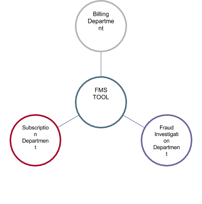
It must be noted that a successful FMS is not to be solely used by the fraud analyst; it must also be used elsewhere in the business process (figure 3) and be able to fit into the whole fraud management scheme. Suggestions to which department has control of the FMS include finance departments, security departments and customer care. It is an obvious implication that all groups should have a role in the use of the FMS, especially if there is a company wide policy dictating response to fraud.
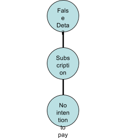
Figure 4 Subscription Fraud
At this juncture it is important to specify the type of fraud that the project will focus on detecting. Due to the shear number of different types of fraud available to study, it is important to concentrate specifically a single type of fraud for this project.
Fraud that occurs from the customer perspective, such that a developed system will detect when a customer is making fraudulent use of the operators network with means and method like Call Selling, PRS abuse and other Non-Revenue Fraud. These are normally related to the modes surfing (figure 5) and subscription fraud (figure 4), since either way uses methods to evade payment structure of the network operators.
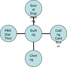
Figure 5 Suring Fraud
Reports suggest that at least 50% of operators' losses due to fraud are caused by "Call Selling", "PRS Abuse", "Internal Abuse" and "Non-Revenue Fraud" (All three will be collectively referenced as Call Selling from now on) 26 . It is important to note that even though it may be a customer who is caught defrauding the network, it may in fact, be an internal problem, with employees supplying external "agencies" with commercially confidential material.
It is import to find where call selling fits into the 4m's classification and also where it fits into the four stage fraud management scheme. Call selling is normally detected as a by-product of monitoring customer use of the network; and since the fraudulent customer is already on the network, we can say straight away that our fraud management stage 1 (prevention, figure 2) has failed. Therefore, anyone who has been caught fraudulently using the network can be said to have bypassed the subscription fraud detection process, since they would have either applied to use the network with false details, or with correct details but no intention to pay for the services used.
Indicators to an active subscription fraud can be identified by checking that the customer is who they say they are. Checks are normally carried out to identify the background information that the customer supplies are valid; these can consist of voting registrar checks, credit application checks and previous address checks. Systems also exist that can cross-reference a customers applications with customer applications of other companies to find consistencies and inconsistencies between the supplied details.
Therefore, we can go through the four stages of the fraud management lifecycle, and amend the subscription process. Unfortunately detecting that someone intends to defraud the network by checking subscription details is never 100% successful (as they might have used legitimate details but had no intention to pay for the services), so the next process is to detect when fraudulent use of the network occurs. Once fraudulent methods have been identified, the company can amend the system to help detect the use earlier. Since this is always going to a be reactionary process, the earlier you find the fraud, the earlier you can put a stop to it and the more money will be saved.
This is where establishing when call selling is taking place requires a FMS (Fraud Management System), due to the volume of call data generated whenever customer use their phone system. There are several accepted ways to detect fraudulent use of a telecommunications network, these include 27 :
- Matching a user call usage pattern to a know pattern that fraudsters use.
- Establishing that there is sufficient change in a customer's usage pattern to warrant investigation.
- Ascertaining if a customer's usage profile has exceeded set limits defined by the fraud analyst.
Firstly if the telecommunication company is well established, then they are more than likely going to know the call patterns associated with fraudulent use. Therefore, one can assume that if a call pattern is the same as an established fraudulent pattern then the customer account the call pattern belongs to warrants further investigation.
Unfortunately, things are never actually this easy. Fraudsters understand that to be able to defraud the telecommunications companies in the future they must evolve their cunning methods, as they also know that telecommunications companies are not stupid and will spot when particular frauds are occurring. Likewise, the telecommunication companies know that to keep the fraudsters at bay they must constantly evolve their methods of detection and prevention. It seems like an appropriate analogy would be that of a two horse race, with the fraudster always one step ahead, so when the phone operators catch up, the fraudster will step up an extra gear and move ahead again.
Some of the tools that the fraud analysts can use when detecting fraud can be summarised as follows:
- Rules based systems: Based on knowledge obtained from experts in telecommunication fraud, the fraud analysts will create a set of rules that will try to match certain aspects of a customers profile with a set threshold.
- Bayesian Knowledge Networks: A graph of related events is created and between each is an arc based on the dependencies of one event on the another. We could then build up a solution from evidence presented to the network based on conditional probabilities. Unfortunately, this needs a professional in both telecommunication fraud and Bayesian Belief networks. Without going too in-depth this solution has been proven to be less reliable 28 , than other methods.
- Neural Networks: Based on past data, a Neural Network should be able to classify and ascertain if an input pattern matches or has enough similarities to that of a pattern which the network has already learnt 29 .
Rules based systems 30 31 32 : Rules Based system require knowledge of the exact parameters of fraud. In addition, since there are seemingly unlimited methods to defraud via call selling, it would imply that the rule set required to capture the fraudsters would also need to be sufficiently large. This is not feasible considering each check may take a finite period of time, and the larger the rule set the longer the checks will take and for possibly little gain in fraud detection rates.
Imagine that there was a system developed to check customer accounts against 500 rules, now imagine that a group of fraudsters establish a new method to defraud the phone company. After a couple of weeks/months the company becomes aware of these methods and adds new rule to handle to this new fraud, however they have a 500 rule limit and need to drop of some other rules. How do they decide which rules to remove without making themselves susceptible to the older methods of fraud? Do they assume that no one will use the older tricks? That would be stupid, since they would be neglecting the opportunist fraudster who might only know the older methods.
Additionally, rules systems are not dynamic in their nature, they normally consist of checking the parameters of customer accounts against threshold values set up by the Fraud Analyst. Therefore, the rules may miss the fraudsters who have not managed to get themselves to the levels where their call patterns are deemed fraudulent.
Rules based systems are also open to internal abuse, since a person looking at the rule set could easily discern its internal workings. For instance if someone knew that if they kept the average cost of each call below £5.00 then all the fraudster has to do is make sure that their average call cost around £4.50. This is an overly simplistic example, but effectively highlights some of the problems with rules based systems.
Bayesian Knowledge network systems 33 34 35 : The parameters of fraud are know to the telecommunication company based on certain features ascertained from the customer base. The fraud analyst would then set up relationships between each piece of knowledge and associate a probability that given a piece knowledge, how much that particular piece of knowledge influences the event B, the event being in this case is the probability of the customer being fraud. For example given that the average call duration is x and most calls occur in the evening, is the customer fraud?
Systems have been researched that use two belief networks. The first network is modelled by the fraud analyst with the relationship between knowledge being established based on previous fraud that has been detected. The second is a network that is automatically generated from all the clear (non fraudulent) data in the network and a network is normally created for each customer class 36 . The data for each customer is then passed through both networks and results from both networks are considered on containing a belief of how fraudulent a customer is and the second a belief of how clear a customer is.
However, what if the fraud analyst missed some important relationships out when inferring knowledge in the system, how would the system respond? What if the customer was perpetrating a new type of fraud that had never been modelled before? My assumption is that the networks would not be able to respond sufficiently. For instance, if the customer simply never intended to pay for a bill, but the calling pattern was similar to one of average Joe customer.
Bayesian belief networks can be used to generate a better understanding of the customer base, by helping the fraud analyst discover relationships in the data that they might have otherwise missed. Michiaki, Taniguchi states that other methods of Fraud Detection exist which provide higher degrees of true classification rates, with lower false positive rates.
The Neural Network 37 38 39 ; Michiaki, Taniguchi have shown that Neural networks are the better at classifying fraud than the previous two methods (rules based and Bayesian knowledge). Depending on the construction of the Neural Network, rates of 85% classification with out a single mistake have been recorded.
What is a Neural Network? Kevin Gurney states:
A Neural Network is an interconnected assembly of simple processing elements, units or nodes, whose functionality is loosely based on the animal neuron. The processing ability of the network is stored in the interunit connection strengths, or weights, obtained by a process of adaptation to, or learning from, a set of training pattern.
Simply, given an input pattern, the neural network will discern from past training what class it assumes the pattern belongs. Essentially, during training each of the nodes in the neural network build up weightings to specific features presented in the training data.
It can be seen that a neural network tries to imitate the reasoning process of a human expert; where a human would build up an image of the solution by combing evidence and weighting each piece against knowledge against the experiences of similar problems. There may be many factors that a human will use to decide the best solution to a problem.
Unlike rules' based fraud detection methods and Bayesian belief networks, neural network will not need a fraud analyst to establish the reasoning the relationships between customers being fraudulent and the attributes, rather the fraud analyst will need to classify the customer accounts based on whether they think they are fraudulent or not. For the network to be able to classify data with accuracy, the data that it needs to use has too be of a good quality, if no relationships between features of data can be established then it may be unlikely that the network will be able to describe the weightings of the features in its internal system.
Neural networks are often use in data modelling or statistical analysis in problems where there are many nonlinear relationships. For instance, weather forecasting, financial forecasting and fraud detection. This is because neural networks have been shown to have an innate ability to classify non-linear problems. It may be good to show how this can be inferred in fraud with an example 40 :
If we look at two variables Number of Calls and Average Call Duration, with each point being a customer (see figure 6A), we have no way to draw a straight line between the two classes (fraud –red, and clear –black). Things start to get harder when we add more variables in and the number of dimensions increase (figure 6B) when drawing a hyper plane between the classes becomes nearly impossible.
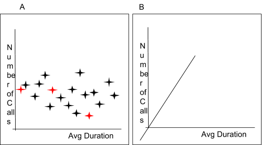
Figure 6 A) Non-linear problem separation B) Added Dimensions
Neural network technologies are commonly used in pattern recognition precisely because they are good at solving non-linear problems, where there may be a pattern that can be discerned but it is very hard for us humans to see them. The more dimensions we have, the harder it becomes to separate each class of data with a line, plane or hyper plane.
Neural networks offer several other advantages over the two other systems of fraud detection (rules based and Bayesian knowledge). They also have the ability to generalise a solution; that is classify how it thinks a particular customer account is in relation to fraud. The customer account information does not have to exactly match the data that the neural network has been trained on. This can be good for detecting fraud that is not being perpetrated in the same manner as other fraud, but has similar characteristics. 41
Another case for neural networks is their ability to adapt to changing circumstances. Not only do they have the ability to generalise, they can also be retrained (once a sufficient training regime has been put in place) with new data, so if the fraudsters evolve their methods, then the neural network can be easily adapted to accommodate these changes, with little extra effort from the fraud analysts.
Neural networks suffer less from the problems of internal fraud attacks against themselves than other methods of fraud detection do. Neural networks have been considered to be black boxes, you supply data to the network and you get a response with out knowing specifically how the network came to its decision. Rules systems and to some extent Bayesian networks, are susceptible to internal fraud, in that a user of the system can infer the criteria used to establish if a customer account would be flagged as fraudulent quite easily. Because simply looking at the nodes of a neural network will not give any evidence as to how the neural network classifies its data, it would require a professional with masses of experience with neural networks to be able to assume any information describing the reasoning process. Therefore, in this sense the neural network is more secure than other methods of fraud detection. 42 43
Once the neural network has been trained, then the process of reasoning if a customer account is fraudulent, is very efficient. The reasoning process (internally) normally consists of matrix multiplications which can be carried out very efficiently. The most time consuming issue with the solution would be summarising the customer account from a database of all customer call information, which is a standard operation across each of the methods described in this chapter. Once the data has been summarised, it can be presented to the neural network and a response will be given almost immediately. Compare this to having to first summarise the data, and then trawl a rule set and compare each rule against the data. A rules system is effectively systematically analysing every customer variable for an account. This process can be more intensive and thus slower than the neural network method.
7.5.1 Why Call Pattern Analysis is not always enough
Call pattern analysis is not the only method of fraud detection that should be employed in the telecommunication industry. If we are having to capture the fraudsters when they are using the network, then they already have evaded out first check (ascertain who they say they are). Also the fact is that the customer may mimic a normal person, and then neglect to pay the bill after the second month. For instance, if we tie the system into the billing departments systems, we may notice that a person might say they are a company, run lots of international calls through it like a large company might, then close down when payment is due. What is to say that the company did not fold on purpose?
7.6 Consideration of Real Time Methods
Part of the emphasis of this project is to investigate Real Time methods used in Fraud Detection within the Telecommunication Industry.
There are two types of real-time behaviour in computer systems, HARD real time and SOFT real time, these are said to be "Traditional Real-Time Systems".
Hard real-time systems are normally associated with Hardware based systems, where the timing of the responses from the software controlling the hardware needs to follow strict guidelines with respect to response times. Hard real-time systems have to be predictable to ensure that timing of event and response actions are always known and adhered to,
Soft real-time systems on the other hand deal with timing requirements in more of a lackadaisical manner, where events timings are non-deterministic. Thus the programming for such system is said to be more complex than its Hard real-time partner.
A more commonly used meaning of "Real-time Systems" is "the successful achievement of results with acceptable optimality and predictability of timeliness". This is the definition that I intend to use through out this project.
I intend to develop a prototype system that once it has been presented with the relative information regarding customer call details a response will be return near instantaneously, hence the "Real Time" part of the project title. 44
8 Identification of Problem and Specification
A customer would come to the software company with a set of requirements. The development house would then analyse the problem domain, propose a solution using certain formal methods and then if the customer is satisfied, they would agree to the design and the implementation would follow.
This project has taken a different direction; I initially identified a problem in an industry and proposed to find a solution to the problem. Therefore, I have also had to take on the task of the customer. This required in-depth research into the industry. In figure 7 the normal model of systems development has been shown. This method has been amended (figure 8) to accommodate this project. 45
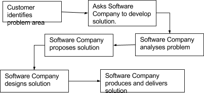
Figure 7 Normal Linear Sequential Model (Waterfall)
From now on, this project joins with what could be considered a normal software engineering project (removing the analysis stage, as it has already been done).
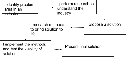
Figure 8 Amended Linear Sequential Model (Waterfall)
8.1 Specification
From the research provided it can be shown that a system to detect "Call Surfing" by methods such as "Call Selling" and "PRS fraud", will help save the telecommunication industry potentially millions of pounds per annum. The proposed solution can be summarised as:
Develop a prototype system using neural networks that will analyse the call patterns of individual customers, returning a status of whether it thinks the call pattern is fraudulent or not. The results of which will ascertain if such a solution is valid.
Using the above criteria as a starting base, we can see from previous research (chapter 7) it is more complex than what is simply stated above. The development aspects of the system can be broken down into the following stages.
- Develop a customer call generation tool. The tool will model how classes of customers behave given user defined parameters.
- Model neural networks using the generated data mentioned above, with a training regime, testing methods and validation of results.
A customer call generation tool will need to be created as I am unable to obtain any proper call information from telecom companies. The customer call generator will be able to generate all the customers and their calls needed for this project.
8.2 System Tools Research and Requirements
The aim of this section is to understand the reasoning behind the selection of the tools used to develop a system that can detect fraud, as well as a further discussion into the requirements of the project. This is essential since we now know the minimum requirements for the solution and before we can design how the package as a whole will work, we must build up a more concrete set of requirements and we must also understand how the development environments will help and hinder development.
The requirements of the system can be broken down in to two separate stages, one for the CDR Tool and the other for the neural network. The requirements were established by myself to give limits to the project, these limits are then imposed to stop feature bloat and to minimise the risk that the project would not get completed in time. The project would have to meet these requirements to be judged successful.
The requirements were gathered after the research stage (sections 7.2 -7.5) into fraud, the telecommunications industry and fraud in the telecommunications industry. Following on from this, several theories and methods of using a neural network presented themselves as possible solutions to the problems; for various reasons where decided not to be implemented. What therefore follows is the final set of requirements deduced from a subset of all the initial theories. These theories were based of and developed in tandem with the system tools research. (Notes available on request)
Since this project is an investigation, it requires the development of a prototype tool. Prototypes as the name suggests, do not have to be a fully functioning product that it is aimed at the people who are to use it. Instead it is a proof of concept, saying that "Yes this solution is viable and will work using following the principles".
It would be ideal to have development tools that are perfect for the task in hand, however unfortunately this can never be the case, for many reasons not only including a limited range of software the university posses, but the cost of the software that I can afford.
8.2.1 Further Requirements for the CDR Tool and Development Tool Research
When considering the features for a CDR (Customer/Call Detail Record) generation tool it is important to understand all the data that is pertinent to a call. This is needed since the analysis of the data will result in the creation of the detection methods which directly affects the success of the fraud detection tool.
The CDR (Customer Detail Record) Tool must be able to create groups of customers that follow a given model. This implies that the models must be able to be specified in a form where the data can be represented in such away that it makes the model information easy to use from a human perspective, but the format of the data is flexible enough so that algorithms can be easily developed to create the customer information.
Customer attributes will be considered in the design section of this project, as further research is needed to judge which attributes are the main drivers of a customer's account information, while other attributes may be inferentially obtained from the main attributes.
Due to the huge amount of data that will be needed when creating a suitable system to model CDR's, it is safe to assume that a RDBMS (Relational Database Management System) will be needed. The main question is: What type of RDBMS should the project use?
Points such as interoperability with programming tools, data extraction facilities, and performance must all be understood.
It is widely considered that SQL is the de-facto standard for information extraction from an RDBMS, so there is little argument that a tool must be able to communicate directly with the database using this Declarative language. 46
Figure 9 Standard model for database communication
Tools for each stage (Generation of data and Fraud Detection System) must be able to communicate with the RDBMS (figure 9). It is here where a remote communication protocol called ODBC (Open Database Connectivity) developed by Microsoft 47 should be highlighted. ODBC allows any program to access RDBMS's created by many different vendors, with little or no need to alter the client application if databases were to be changed during the project. ODBC also removes the distinct of where a RDBMS is physically located, as it does not require the client application to implement any network communication protocols.
Because of the decision that ODBC will be used, we are essentially free to choose whatever RDBMS is available. The options for RDBMS are as follows, but not an exhaustive list of all the database systems available to use:
- MySql, a highly used, efficient multi-user open source RDBMS, used on many websites throughout the internet. However, several failings remove this choice of RDMBS, from the running. These include (at the time of assessing the requirements) no support for sub queries (link), limited join facilities (link) and no support for SQL views. 48
- PostgreSQL is a heavy weight multi-user open source RDBMS alternative to Oracle. With excellent performance and uptime, inclusion of its own SQL style procedural language to enable easier data manipulation, and competent ODBC drivers. Has the ability to run in a windows environment, but still requires ODBC to connect with it. 49
- Oracle, a heavy weight business class RDBMS with excellent performance and scalability. The likely feature set required for this project will not cover even ½ of the available features that Oracle offers. Oracle has had for many years its own data input language called Oracle Forms as well as it's own procedural language. While I have worked with Oracle in a professional environment, it is judged that for this project its functionality is an overkill. Combine this with the fact that the Oracle DB will always reside in the university servers and access to such services may for some uncontrollable circumstances become unavailable. 50
- MS Access 2000 is a business orientated RDBMS, although it does not support many of the higher end features of some of the other commercial databases such as efficient multi user support.
MS Access 2000 has its own implementation of VBA (Visual Basic for Applications), which supplies a far superior interface and development language than the other RDBMS mentioned through the use of Windows forms allowing for easy prototyping and application development; partly due to the ability to model, control and access the data types and the underlying data store with no extra work. 51
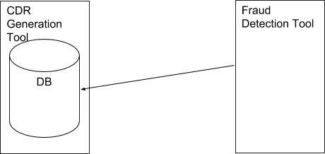
The ability for MS Access 2000 to have the CDR generation tool sitting directly on top of the RDMS is a tremendous advantage. As keeping everything in one location will enable me to develop the software in more than once place, rather than establishing connections to remote databases which could prove to be cumbersome, slow and prone to failure (depending on the internet connection). (Figure 10)
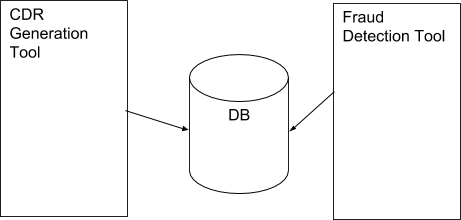
Figure 10 An Ideal situation for CDR Tool and Fraud Detection Tool
8.2.2 Further Requirements for the Fraud Detection Prototype and Development Tool Research
On the Fraud Detection Tool side of the requirements, we have to choose a tool that has the ability to access the data store, the ability to perform extra processing of the data and show the results of the tool's performance. Like previously mentioned, the tool will simply be a prototype, proof of concept as such and therefore will not require a user interface that would normally be the case if we where to develop a system that has been put out to tender.
The Fraud Detection Tool can be visualised as two separate, stages. Gathering the data from the RDBMS; and processing it with the Neural Network.

Figure 11 Processing the data through a neural network
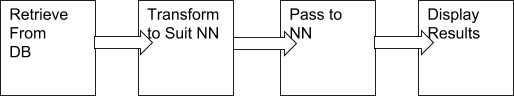
Since the Fraud Detection Tool will require the use of a neural network, there are two options:
- Create a neural network from scratch with a programming language.
- Create a neural network using a tool inside of a package especially designed for prototyping and mathematical work.
It is obvious that the correct choice would be to choose a software package that can simulate a neural network. Since the development of a neural network from scratch would be a separate project in itself due to the many different types of neural networks available, I would have to understand the precise workings of each to ensure they are correct, and doing this would require time that I do not have if I am to create a fraud detection tool.
The requirements for the neural network cannot be as solidly set as those for the CDR Tool, since it is this section which is the research part of the project. To create the final neural network it is a process of making use of many different architectures, different training methods and then combining the results to get a final optimal network.
The design of the neural network and the training methods, along with an overview about neural networks is covered later in the design section of this project.
Luckily, the final neural network must meet several defined requirements:
- It must detect fraud to a reasonable level;
- A final network must be produced, that 'would' be used if the model created apply to what happens in the real world.
- Threshold level must be established to indicate which classification the data is in, i.e. any value above and including 0.75 is clear, whilst anything beneath this value is fraudulent.
After cutting a large swath through the number of potential systems I can create by removing the need to hand develop every neural network system, I can concentrate on developing the prototype by swiftly creating and testing the most suitable networks for the project and establishing which prototype system is more adept at classifying fraudulent customers.
With the ability to swiftly be able to create neural networks, it would be wise to require the system to automate the training the neural networks. Doing this will free myself from having to be involved in the process of creating each network. Once the networks have been trained the system should be able to prune the Neural Networks that cannot classify the results correctly. The nature of Neural networks means we can never guarantee 100% correct classification of the data so we will need some method of visualising the results on completion.
These requirements all point to systems that have either neural net packages included or the ability to install them as an add-on. It comes as no surprise that I am limited to the software that the university has available, these include:
- Matlab
- Visual Basic
- Visual C
There are several tools that aide the production of neural networks, however non that I have found, have the inherent ability to provide statistical functions, data processing, custom function generation and ODBC database connectivity that MATLAB provide. Although it is true that both of the Microsoft Visual programming languages are very flexible and enable rapid prototyping. They unfortunately are not pertinent to the rapid prototyping needed for this project, since many of the statistical functions and matrix operations required for neural network analysis are not provided as standard (Also the quality of neural network packages varies wildly between implementations).
MATLAB on the other hand provides all the data processing functionality required of this project with tried and test neural network packages and ODBC connectivity.
9 Design
9.1 Chapter Summary
This chapter deals with the design of both parts of the system. The CDR (Call Detail Records) Tool and the NN Fraud detection tool. The design is based on the requirements determined during the research and presented in the specification.
This chapter will not deal directly with each algorithm used in the program, it will also not show every data processing stage in detail, rather it will describe the important algorithms used to generate the data; the data it will generate based on model attributes; data that is generated as a consequence to data supplied and generated using input parameters; and an overall flow showing how the system will generate the data for each of the customer in the models.
In addition, because the Neural Network is not a full tool, but rather an experiment in to the likelihood that such a process is practical to detect fraud. Only issues concerning the creation of the NN will be documented. This may include brief discussions in to helper tools used to create the NN and to test the efficiency of the model used. But will mainly focus on the methods used to train and test the network.
The design section is a verbose description of the design process sprinkled with flow charts and diagrams showing the major points discussed. This method of documentation was chosen to give the reader a fuller understanding of the effort involved and the algorithms used. Rough design work can be obtained on request.
9.2 Combined System
The system as a whole must be considered before we can look into its principle components. As described in the specification (8.1), the target of the system is to show that neural networks can be used to detect fraud. This project differs from normal 'stake holder' projects as there are no stake holders other than myself. This
What can be seen below is a very abstract view of how the whole system will work. The first two stages are strictly based in Microsoft Access; the third stage is a shared task between MATLAB and Microsoft Access. Primarily MATLAB uses the ODBC functionality of Microsoft Access to gather information about the customers, however the query generation functionality of MS Access allow better aggregation of the data through the use of Views. Implying that most of the work is then done on the database server and not in the neural network suite, which is the way that all good database driven applications should be created.
The final stages (4,5 and 6 in figure 12) are based inside MATLAB and are there to train the network and decide which network is most suited to our problem.

Figure 12 Abstract overview of data flow in the system
9.3 CDR Tool Design
The CDR is the first major design hurdle that must be overcome when developing the Neural Network solution, which as highlighted in the Research and Specification, real world call data is impossible for me to obtain from Telecom companies.
The role of the CDR Tool is to generate all the call data needed to train, test and validate the neural network models. The theory is that every customer belonging to a telecommunication company will fit in to a certain demographic or customer profile, be they fraudulent or not.
If a telecommunication company had already provided all the information about their entire customer base, we should be able to take a sample of the customer population and aggregate the data in such away that each customer would fit into one of many profiles that we have defined.
Each customer profile group will have distinct attributes that every customer in that group bears some relationship. An example is probably best:
After studying the customer information, we know that there the telecommunications companies customer base represents 20 distinct classes of customer, some of them follow:
- People who use the telephone rarely and only in the evening;
- People who use the Internet regularly at any time in the day;
- People who have friends and family who are based abroad;
- Companies who are shops and stores;
- Companies who are small, but have a national customer base;
- Companies who are large and have customers worldwide.
Each of the customers in each of the classes would not be the same as each other, but their attributes would be similar to each other. As above, customer type one is unlikely to make any PRS call or International calls, but may make local calls to their friends and families. People in this group will not have the exact same calling pattern, but they will have the same attributes.
As you can see if there are enough classes, every customer could be uniquely placed inside the classes.
Following from this it is therefore acceptable to work in the reverse from what a telecommunication company would do when looking at their customers. If we can think of the potential classes of customers, we can then build models that will mimic individual customers based on the classes in which they should fit.
The problem is how to define a model in a way that the customers do not have the same calling patterns, but their calling attributes fit that of the model.
A statistical property called a "Normal Distribution" or "Gaussian Distribution" shows how a population is distributed in relation to a property. It is broadly related to the histogram function, but instead of showing the number of people in each class, it shows the probability of that property occurring, as it is normalised against the sample.
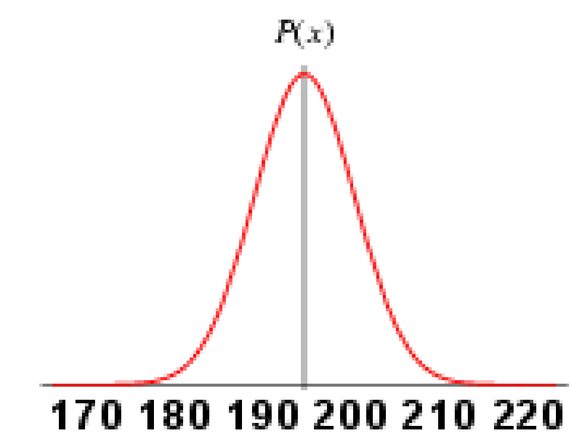
Figure 13 A Gaussian distribution based on male heights in the UK
The height of the curve represents the probability of the measurement at that given distance away from the mean. The graph above represents the heights of men in the UK, who might average about 195 cm. Therefore, the probability of picking a man whose height is 195cm is the highest, while the probability of a man with height of 220cm is far smaller.
As shown, the normal distribution is built by centring the graph on the mean (the highest probability of an occurrence), and can be generalised using the following function. 52
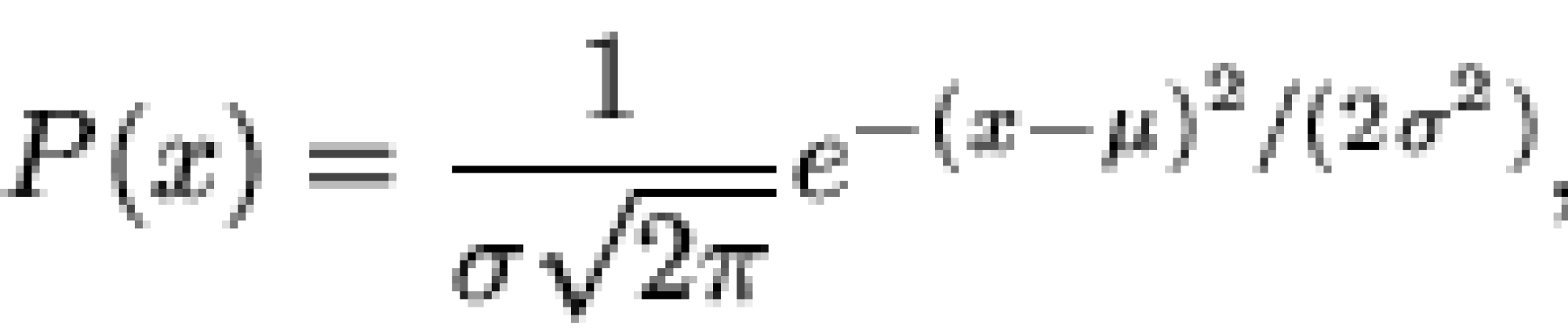
Figure 14 The Gaussian distribution function
Why is this property good for generating Call Detail Records based on models?
Eric W. Weisstein states the Central Limit Theory as having the mean of any set of variates with any distribution having a finite mean and variance tends to the Gaussian distribution[sic]. In essence what it is implying is: real data never actually will follow the mathematical ideal of a Gaussian distribution, but many types of data distribution can be said to broadly follow a Gaussian distribution. 53
This is good, as it means that we can use this principle by assuming that when a class of customers is to be generated, everyone in that group will differ from the mean by a random amount within a limit defined by the distribution. Nevertheless, the majority of people will tend towards having the properties similar to that of the mean.
What therefore must follow if we are to generate customers that randomly differ from each other, but follow a Gaussian distribution; is a function which can generate numbers that are normally distributed.
Several properties exist that a when generating a distribution following a Gaussian distribution, these are the mean and the standard deviation. The mean has the effect of centring where population will be based around, and the standard deviation will affect the spread of the population. A higher standard deviation will state that the further outlying values have a higher probabilities of occurring than normal, thus squashing the graph.
What can be seen in the following two charts, is a Gaussian distribution each with the same mean, but the standard deviation in B is larger than that of A, thus having the effect of the P(x) at the mean is smaller in figure 15 than in figure 16. The two graphs have been scaled so that they look similar, in height.
Figure 15 Gaussian Distribution A
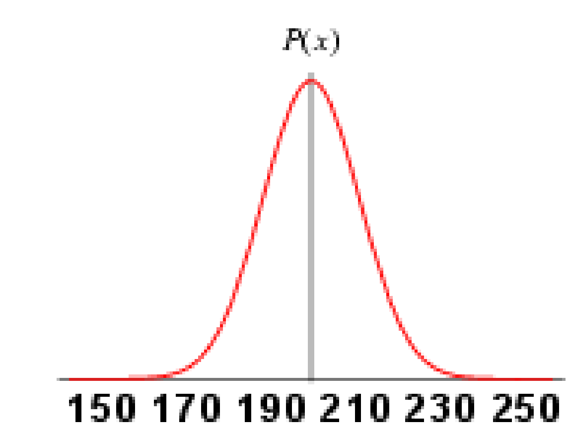
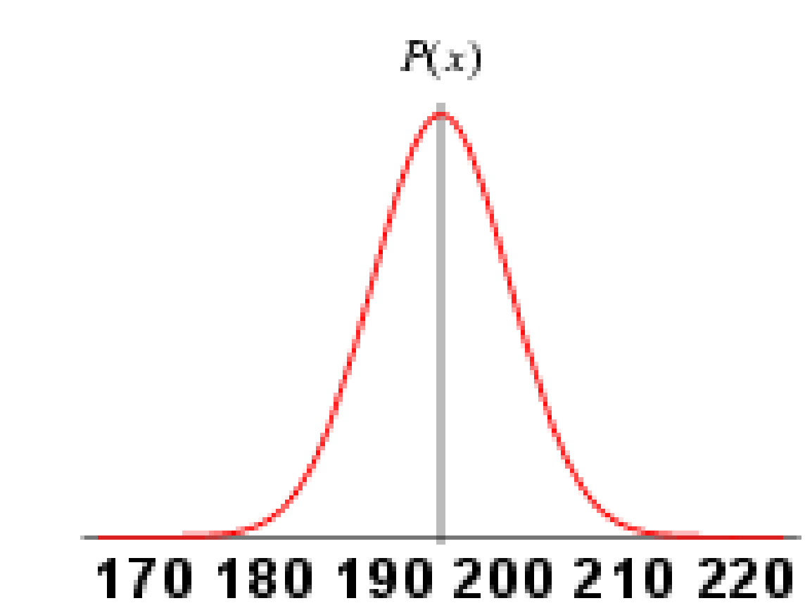
B)
Figure 16 Gaussian Distribution B
Such an algorithm exists that will generate random numbers that will follow a Gaussian distribution. It is called the Polar Box-Muller 54 method and has the ability to generate two random numbers based on the Gaussian distribution of mean 0 and a standard deviation 1 from two uniformly distributed random numbers between 0 and 1 (many programming languages provide functions for generating uniformly distributed random number). It is a simple case of manipulating these two generated random numbers to get them to fit other distributions, such as a mean of 34 and a standard deviation of 5, which would involve multiply the numbers by 5 and then adding 34 on to the result.
Furthermore, it is assumed that each customer in each model, would have a similar style of days (Monday, Tuesday, etc) in which they place telephone calls, for instance it may be that a casual user of the phone, would make calls in the evening or on Saturdays. These patterns would generally not differ from customer to customer in the model, but would follow more of an uneven distribution and thus nothing like a Gaussian distribution. Gaussian distribution are said to only be of use when the variable in question is "continuous" (like peoples heights) and not discrete (like days of the week - Monday, Tuesday etc - or call types such as PRS, Free, Local etc).
Therefore, a method that allows weights to be assigned to each discrete variable needs to be developed. A solution exists based on the process of biased weightings. For instance when tossing an unfair coin, it could be said that the heads side is unfairly biased (i.e. it is more likely to lands heads up).
The method will pick a random number between 0 and 1, then using the weighted probabilities it will asses which property the random number belongs to. An example:
A set of three discrete properties exist (A, B and C), A is twice as likely to occur as B and likewise with C. Such that A = 50%, B=25% and C=25% where A+B+C = 100% as seen in figure 17. Our random number generator produces an even spread of random numbers (every number will occur the same amount of times given enough attempts). 55
Figure 17 Biased Weighting
Therefore, if the number random number is >=0 and <0.5 it is a class A, >=0.5 and < 0.75 class be etc. This indicates that together B and C should occur the same number of times that A occurs, with B and C occurring the same amount of times as each other.
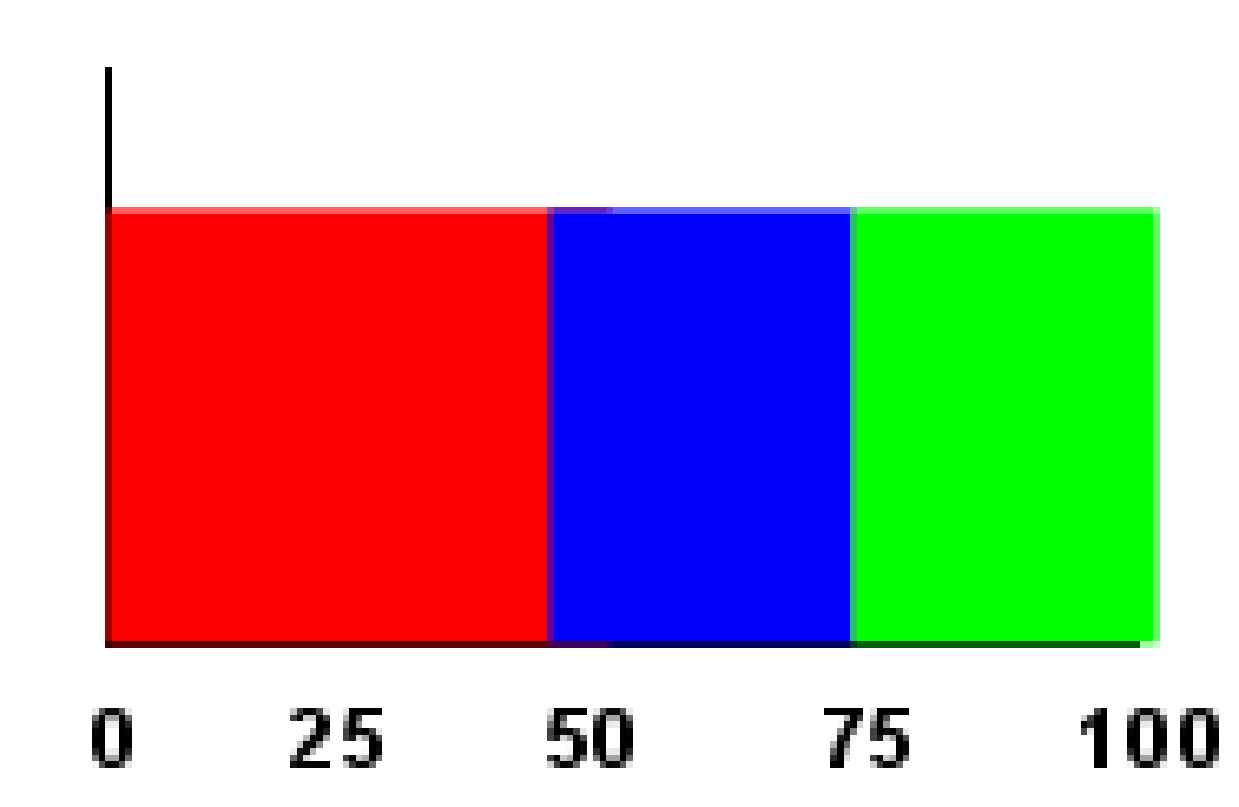
Now that we have the functions to create the Gaussian distributed random numbers as well as biased numbers, it needs to be decided what properties of a customer account are the affecters of the call data. An example will provide a better understanding of what is meant:
The cost of a customers monthly bill, could be said to be random but each customer in the group will have similar bills. However, the cost of the calls is not the effecter; it is the average duration of the calls, the types of calls being made and the period (off peak, on peak). The cost of a call is a function of these properties – y=f(call period, call duration and call type).
When considering which inputs should be based on a Gaussian distribution, the following call parameters are good examples, as normally what is held in a Call Detail Record is the type of call, the start of the call, the end of the call and the cost of the call.
Other attributes which do not need to follow a Gaussian distribution, for instance each model, will contain the probability that a particular call will happen on a set day (Monday, Tuesday etc).
Each attribute that is said to follow a Gaussian distribution will need to specify two variables, one being the mean (where we want our population for the variable to centre about) and the other being the standard deviation, which will say how much on average each of the elements differs from the mean or the spread of the data. The other attributes that need to be randomly generated but following a set weighting, need only have there weight established and scaled to 1 in relation to the other variables in the set.
Attribute affecters are the attributes that will have a direct affect on other attributes; these attributes are therefore the ones that will be specified when considering how each of the models is generated.
Attributes such as call cost and average call cost do not need to be generated when each customer is being created; rather they are produced as a consequence of other variables. The call cost would be established by assessing the time period that the call was made, considering how long the call was and also dependant on the type of call made (PRS, International). Table 2 documents all the call parameters that the CDR Tool will have to model.
Table 2 Call Parameters for the CDR Tool
|
Call Parameter |
Distribution Type |
Description |
|
Call Type |
Weighted, Discrete |
There are discrete number of different call types available (Free, Local, National, International, PRS and Mobile), within each customer class it is assumed that the attributes of the call type are similar for each customer. The probability of each type of call occurring is then established. |
|
Average call duration compared to the population |
Random, Gaussian |
Each customers average call duration will be different from other customers, but again they are expected to be in a particular group class, because the average call duration for each call type is similar. Each customer in the group will have a similar spread to the duration of each of the calls. |
|
Average Call Duration |
Random, Gaussian |
Each customer's calls will not be the same duration as every other call they make. However, their calls will be of a similar nature, for instance local calls made might average 5 minutes, but vary from 1 minute to 7 minutes. Averages might vary depending on the time of the call, since people are more likely to make off-peak calls than on-peak calls. Average Call duration is established by the random number generated from the "Average call duration compared to the population" variable |
|
Time of call |
Weighted, Discrete |
People are expected to make calls any time of the day, however the likelihood that they will make a call at 3am is far less than the probability of them making a call at 6:30pm. The distribution is not continuous, but can be separated into discrete time segments. |
|
Call Day |
Weighted, Discrete |
Like the time of day when a call can be placed, each customer class can be expected to make more calls on certain days than others. For instance, a small shop's busiest day might be Saturday, while on Monday the shop is closed to allow the staff to have a weekend. Therefore, the probability of a call occurring on Monday for that customer is nil. |
|
Number of Calls made |
Random, Gaussian |
Each customer in the specified customer class will have the number of calls they make for each period similar to that of the other customer in their class. Each of these based around a mean number of calls made each varying from the mean by some random amount. |
|
Number of Calls Received |
Random, Gaussian |
Like the Number Of Calls Made, the Number Of Calls Received for each customer in the group will be similar to each other, varying by a random amount. |
|
Number of the Calls per call type. |
Weighted, Discrete |
Every call that a customer makes will not be a random call type, rather the calls will be spread out over the different call types (Local, National, International, Free, PRS and mobile). A normal customer is going to make hardly any PRS calls |
|
Number of telephone lines |
Random Gaussian |
Every customer will have one or more telephone lines, if the customer is a company they are normally going to have many phone lines, if only one line was modelled (and since calls cannot overlap) then the times of the calls would not be accurate and therefore the costs of calls would also not be accurate for that model. The number of telephone lines will follow a Gaussian distribution, with each customer having the number of telephones randomly dictated by the distribution of the population. Households will normally only have one phone, but they could have two lines. |
To make the design of the CDR Generation tool easier, some assumptions have to be made:
- Once a call starts, the billing period the call starts in is the billing period the call is charged for. If it started at 7:59am and 8:00 am is when the on peak billing started, the whole call will be classed as an off peak call.
- Calls in this model will always start on a 5-minute boundary.
- The granularity of the received calls will be a day.
9.3.1 Flow of Data When Creating a Model
Rather that give in-depth commentaries on each stage of the model generation and detract from the intent of the project, what follows is a high level description and a flow diagram (figure 18) showing a high-level abstraction of the generation of all the customers inside a model.
- Create all customer Phone numbers and number of calls they can make
- For each customer
- Establish the types of numbers they can call
- Establish phone numbers they can telephone for each of the call types
- For each call they make
- Generate start time and duration
- Check the start time and duration do not overlap any other calls
- Once the calls have been created for each customer. Store the call information in the database.
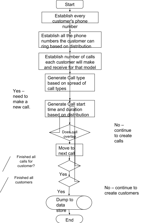
Figure 18 Customer Generate tool flow diagram
9.3.2 Consideration of the UI
In this project the UI is a means to an end; simply put the UI is a shell to allow simple access to the model parameters. This is not an exercise into requirements gathering with respect to shareholders, nor is this project aiming at User Interface design. The user interface for the CDR tool is simply a utility that will help to input model information about each of the customer models.
Therefore, no usability studies where carried out for this project and no task analysis took place.
9.3.4 Data Representation and Considerations
The format in which the data is stored needs to be considered as to allow easy access to the data when it comes aggregating the data for analysis by the neural network.
9.3.4.1 Internal Data Representation
The internal representation of the data in the CDR Tool is an important aspect to consider. The quality of the data representation will have effects on the overall success of the project. Incorrectly defined data requirements and specification will have a knock on effect of not allowing the neural network to use the data that will enable it generalise efficiently. The input requirements to the neural network will be discussed later in the report when considering the neural network design, but the data access queries that will generate the data will be shown in this section.
9.3.4.2 Customer Information
Each customer needs to have an account. Within this account, data needs to be stored concerning the model that was used to generate this information and the status that is assigned to them (fraud/non-fraud).
Following from this it would be useless not to have information about each call. Including such items as call start time and end time (including the date of the call); the type of call (Local, Free, National etc.) and call cost; and also needed would be the number that was customer was calling.
Additionally needed is information about the number of calls received during the period. Each call that is received only needs to store the date of the call. This is due to the decision not to use a lot of information pertaining incoming calls when considering what the neural network will use.
9.3.4.3 Entity Relationship
The data is partially normalised to first normal form. This is partly due to speed aspects of the system as well as some repeated data being kept in a table; this includes items such as start data and end date, which could be represented in another table, but would then require extra joins, which would slow the system down dramatically.
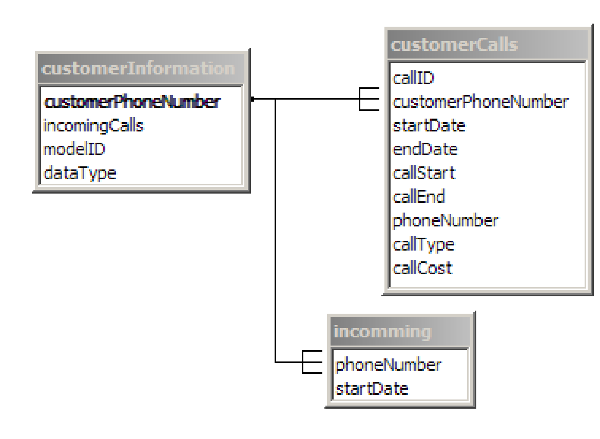
Figure 19 Basic Entity Relationship for customer information
The customer information is first created with information such as their phone number; this phone number is then used as the unique identifier in the remaining tables. For analysis sake, the modelID which was used to create the customer is also stored.
The remaining tables hold information pertaining the calls that the customer makes such as the start time, the end time, the cost of the call, the phone number that was called and the type of call that is being made.
Incoming call information is also stored, but only requires information about the phone number that called the customer and the date on which the call takes place. This is because very little information pertaining incoming calls will be used in the final network and no further analysis of incoming call patterns will be needed for this project
9.3.4.4 Data Access
Data retrieval is an important part of the system; if the data cannot be aggregated easily then it is practically useless. The system needs to be able to generate the information needed by the neural network as to allow the neural network to be able to understand the features in the data that result in correct classification.
What follows is a brief look at the final query used to pull all the data out of the database. This is a visual representation of the query, rather than an SQL code representation. It must be noted that this query pulls data from other queries. These external queries can be considered as "views" in SQL relational database speak. They are present for brevity as not to make the final query overly complex with the masses of joins that it has to perform.
All the queries used in this project can be viewed in the Microsoft Access 2000 Database supplied on CD in the appendix of this project.
The query shown in figure 20 is the main query used by the neural network software and gathers aggregated data about low risk calls and high risk calls over a two week period.
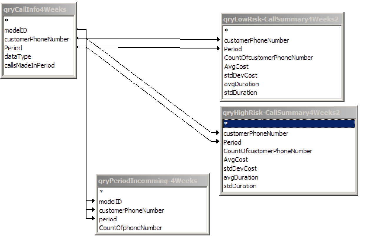
Figure 20 Overview of tables, fields and relevant joins used in the final output query
Descriptions of the queries used can be seen in the appendix (16.2.1)
9.3.4.5 Index Considerations
When considering which indexes should be present on a table, there are some well established guide lines that can be adhered to, to allow for efficient access to the data:
- Any field that is used in a join operation
- Any field that is used in a where clause
- Any information that is suitable unique throughout the data
- Any information that may be used with aggregate function such as Avg, sum etc.
The following indexes have been applied to help speed up access to the database.
9.3.4.6 Aggregating the Data
When considering telephone records, it is important to understand with respect to pattern analysis, the time span in which the data should be aggregated over. Too coarse a granularity of the time span may mean that suitable patterns for fraud detection may not be able to be noticed, while too broad a time range has the potential to catch the fraud but will be too late to take any preventative action against the fraudsters. In either the case the Fraud detection tool would be considered to be useless.
The time period which has been chosen for this project is two weeks, however this can be changed with very little effort. The reason for this decision is based on the fact that billing normally occurs once every month and a system which waits this long to capture the fraudster will be unable to catch the fraudster who defraud the operator for the first month and then leave. A feature called sliding windows can be used to help capture fraudulent new customer to the company.
Sliding windows (figure 21) can be seen as the effect of having a view on to a certain portion of the data, in this case we might consider it to be customer phone usage. The window is a set width and does not cover the whole of the data set. Each of the data in the window is analysed and used. Next we move the window (or view) slightly along in the data set, doing this we can then build up a day by day summary of two weeks of customers usage.
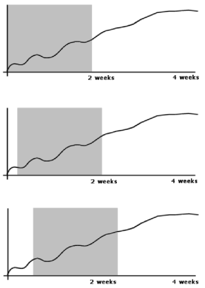
Figure 21 Sliding Window Effect
Now if we have a window the size of two weeks, we can analyse this information nearly as soon as the customer has arrived on the network (by the end of the second week we have a good start for monitoring their call patterns). Once the first two weeks have been analysed we could then set the window's starting position to that of the 2 nd day of the first week and analyse the customer account again up to the 1 st day of the third week (15 th day). This would then occur each day for the customer.
This methods shows that by the end of the first month we have been able to analyse 14 different combinations of two weeks worth of call data. By the second month we will be able to analyse at least 30 full combinations of two weeks worth of call data. This is better than simply analysing the customers accounts once every two weeks or once every time the customer is to be billed.
9.3.4.7 Storing the Models
The models must also be stored in the database to allow the creation of the customer detail records. Again, this is normalised to first normal form to reduce the number of columns in each table to ensure that they are easy to operate. All of the parameters used on the forms are stored in one of these tables. Information relating to off peak calls is stored in the "off-peak" table; data relating on-peak call in the "on-peak" table and other information in the model table.
9.3.4.8 Testing the Model Generator.
Testing a project is an important step in the lifecycle of a project, if the project does not meet its requirements or it does not function correctly (i.e. breaks) then the people who need it will not want the program. If the code in an investigation such as this does not work, then it is likely that the results will be incorrect and the final outcome of the project will be wrong.
Testing a project normally takes the form of two different stages:
- To ensure that project meets the requirements
- Functionality testing to ensure that no bugs have been introduced into the code.
Requirements testing normally takes the form of black box testing and functionality testing takes the guise of white box testing.
Black Box Testing can be considered as testing without information of the internal workings of the program being tested. For example, the tester would only know the allowed input parameters and what likely outputs should be returned, but not actually how the program arrives at the result.
Black box testing can be considered to be testing with regard to the specifications; no other information about the program is required such as code listings. Therefore, the tester and the developer can be independent of one another and thus avoiding a programmer being biased toward his own work and adversely effecting the testing.
White box testing is testing with full knowledge of the internal workings of the program being tested. The tester in this instance would normally be the programmer and would know the code paths that a particular piece of code should take. White box testing is used to check for robustness of the code
Because the output will not always be the same for every run of the CDR Tool, testing is a bit harder than normal. Therefore, unit testing took place throughout the development of the CDR Tool. This meant hand testing each major functional requirement, which is essentially black box testing.
Of particular interest is the random number generators used. Since they are not simple random number generators, code had to be developed to make the random numbers either follow a Gaussian distribution or follow a weighted distribution.
Black box testing has been chosen for this project. Normally with the black box testing the programmer/designer and the tester are normally independent and have no contact with each other; however, this cannot be the case for this project as I am the only person in this project.
The test have been designed around testing if the CDR tool can correctly generate the call models; this implies that the random number generators are known to function correctly and within given parameters. Therefore, the test plans will not only include whether models have been generated correctly but also test whether the random number generators can produce numbers with the desired parameters.
To keep this project sufficiently short the test plan has not been included in this section; however, black box tests have been included in the appendix Test plans and results are supplied in the appendix (16.4.1)
.
9.5 The Neural Network
The Neural Network is the second stage of the project and is the section that is probably the most important, as the aim of the project is to detect fraud and the NN will be the method used to detect the fraud.
Following on from the research it is important to establish how a neural network functions and what type of Neural Network will be used in the final solution. It is important to model a couple of types of neural networks and then empirically decide which would be the best to use if a full tool were to be implemented.
What follows is a discussion on the training methods used, the Neural Network Structures available for modelling, and an overview of the Performance Analysis used in the project to determine which Neural Network is the best at classifying fraud.
Following on from a discussion about neural networks, will be a brief discussion about the tools created to aid the development of the neural networks.
This is not a tutorial into neural networks, but rather the design of the network presented by showing the major design decisions and why they were taken. This is due to the fact that MATLAB already provides all the tools needed to create and train a neural network. All that is needed are decisions in to the reasoning behind the choices made.
No mathematical proof as to how neural networks work has been provided in this chapter so to keep the project succinct and to the point.
9.5.1 What is a neural network?
A neural net is a system that is set up to mimic the function of an animal neuron. The basic neural network consists of a single node (or one neuron). This node can have many inputs, and normally one output (for a single node). An animal neuron can be seen to operate by summing the electrical signals entering the neuron through the dendrites collected from the synapses, and firing off a signal down the axon if the input signals attain some limit, sometimes called the activation . (Figure 22)
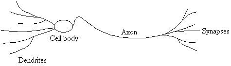
Figure 22 An animal neuron
The artificial node has the weighted inputs (similar to the synapse) from other nodes (or cells); this is achieved by multiplying the input value by a weight value (the weight value essentially says how important the input is). The node will perform a summation of these inputs and fire (or activate) when a certain level is reached. 56
The first artificial neural nodes (figure 23) would simply output a 0 if the activation was not reached or 1 if the activation level was attained, these were known as Perceptrons and used threshold logic units (TLU) which took the form of a step function. This system was okay if only binary information was being supplied and they could tolerate noisy inputs (the inputs not being exactly 0 or 1). However, systems using this were shown not to be able to classify problems that were not linearly separable, such as the XOR problem. The activation level was normally hand set to a value that would give correct classification to the problem. 57
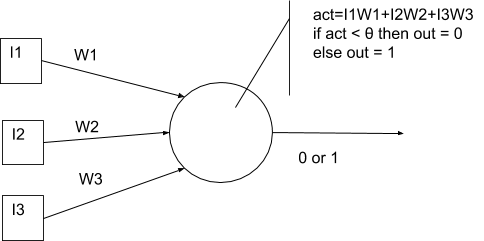
Figure 23 An artificial neuron based on Binary Threshold Logic Unit
Real neurons are not believed to operate in this manner, but rather receive inputs as a continuous pattern of information, which can be summarised as a continuous range mimicking that of an analogue system. This therefore meant that the TLU could no longer simply operate using a step function but needed a function that would output a value signifying which side of the problem domain the solution is in, based on the strength of the inputs. 58
Figure 24 Logistic Sigmoid function & Tan Sigmoid function
Because the data being input is continuous, if we were to use a system such as a feed forward network, which connects nodes to other nodes then the output would also have to be continuous. There are several functions available, which normally take the forms of a bipolar output and unipolar output. A bipolar output (figure 24 - tan sigmoid) is one that takes the range of -1 to 1, whereas a unipolar output (figure 24 -Logistic Sigmoid) is one that takes the range of 0 to 1. These functions can take an infinitely large range of inputs and convert it to a scale of 0 to 1 or –1 to 1 59

Figure 25 An artificial neuron based on a continuous sigmoid output function
If we have data that is non-linearly separable data, how can we find a curve to fit this data? Sigmoid functions such as the logistic sigmoid, can be altered and summated in such a way that we can get them to fit our problem domain (see figure 26) which is could approximate our problem.
Figure 26 Combining logsig(5x-2) + logsig(x+2) – logsig(2½x -12 )
There is no way to know how many sigmoid operations we need to get the solution to fit the curve, and this is where the training of the neural network comes in which will be described in detail later. Suffice to say that each of the hidden nodes will output a value based on its sigmoid-based activation function, the output node's role is to combine these results into something similar to the process of us combing these sigmoid functions as seen in figure 26.
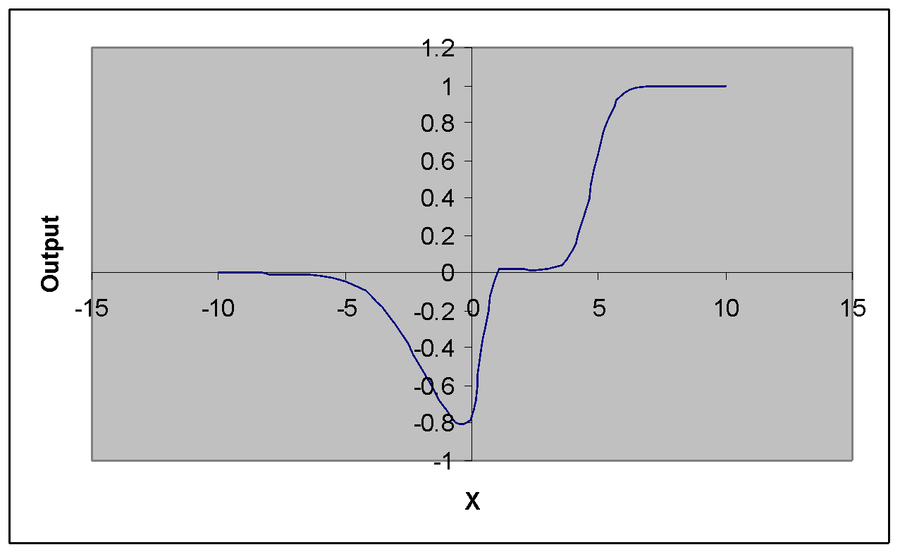
Figure 26 could represent "anything above the line is in class 1 while beneath the line class 2". This is precisely what the neural network should achieve.
This is why some classes of neural networks are good at function generalisation, you train the network with the inputs of a function and after a training session it should be able to mimic the output of the function with out actually knowing the exact inner-workings of the function. 60 Rather it establishes how the function operates through a process of looking at the output of the function in comparison to its own output and adjusting its internal so that it becomes more like that of the function it is trying to mimic.
9.5.2 Types of Neural Networks
So far, I have discussed briefly what a neural network is while mentioning some types of networks, now what follows is a brief discussion of the types of neural networks available.
There are many main types of neural networks: feed forward networks; feedback networks or recurrent network; Self organising networks, the list continues.
A feed forward network operates by passing the output from one layer of nodes to be the input of another lower layer, hence the data feeds forward throughout the network.
Figure 27 The Feed forward Neural Network
The inputs are supplied to the network; the node then calculates the output value based on its activation function and passes it on to the next layer as inputs to the neurons in the layer below. Each node in the layer above can be attached to every node in the layer beneath. Each connection is then assigned a weight and this weight then acts as a "importance level" to the information being output from the node above to the node below. Networks which have every node in one layer connected to every node in the layer below are said to be fully connect. Fully connected networks are the only networks going to be considered in this project for conciseness.
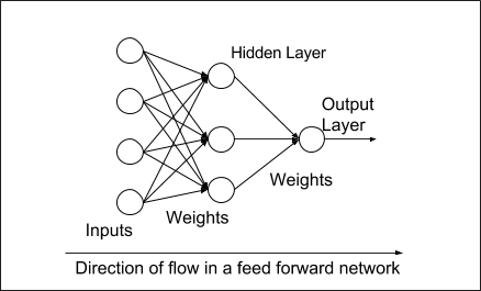
Figure 27 presents a feed forward network known as the MLP (Multi layered Perceptron). The MLP is a good choice and is generally described by many textbooks to be sufficiently easy to implement and understand, but also good at finding solutions to problem domains. 61
MLP's normally consist of an Input layer, followed by one or two hidden layers; hidden layers are so called as we have no direct access to their inputs or their outputs; finally an output layer is added, so that we can gather the results from the network. The MLP can be considered a fully connected feed forward network of Perceptrons with one or more hidden layers using a continuous output function for each of the nodes.
Figure 28 A Recurrent Network
The recurrent network, also know as a feedback network, will have some of the hidden nodes supply their activation to a node (also known as a context unit) in a lower layer, the output from which is then used again in the nodes that supplied the input to the context unit and essentially what happens is a feedback loop occurs (figure 28). This type of neural network is normally used when temporal information is being used, that is to detect patterns that vary over time. Further more discussion of recurrent networks is out of the realms of this project. 62
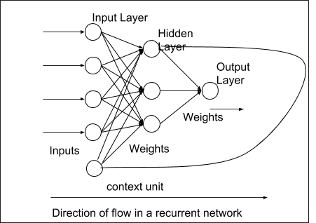
Many other types of neural network exist, but for brevity and simplicity, only the feed-forward networks based on the Multi-layered Perceptron and techniques associated with this will be considered. The number of hidden layers will be set to one, as this is suitable for solving many non-linear problems whist having two hidden layers will increase the number of test networks required and the training time dramatically.
9.5.3 What Neural network to use?
The neural network that this project will use is called the Multi-layer Perceptron (MLP). This type of network is a feed forward network, and will be trained using Back-Propagation.
The network will consist of three layers: an input layer, a hidden layer and an output layer (similar to figure 28), however it is known as a two layer network since two layers work on the data. MLP's can have more hidden layers, but the effort that is needed for training is greatly increased with every additional hidden layer, additionally this design for a neural network, with one hidden layer is sufficient to solve many non-linear problems, including function approximation.
Multi-layer Perceptrons have one or more layer of hidden nodes, there are no set rules to the number of hidden nodes there should be so the best way to determine this is through a process of trial and error. However, knowing roughly where to start (with the number of hidden nodes) has come under consideration.
Carl G. Looney shows that 63 :
- Masahiko recommends K-1 hidden nodes, where K is the number of distinct training patterns. This is not feasible since the number of unique training patters could be as high as 1400 since the data is in continuous form.
- Hayshi shows that , where M is the number of nodes, N is the number of inputs features and J is the number of output nodes and c is some constant. This is more reasonable method and by adjusting c, we can get a range of hidden nodes from 5-10.

A network with too few hidden nodes will not be able to generalise sufficiently enough, while a network with too many hidden nodes may require phenomenally more training cycles to be able to converge on a solution.
The number of hidden neurons in the final neural network will be determined empirically through a process of trial and error. There will be a set minimum (5) number of neurons and a set maximum (10); it is then a simple task of establishing which network structure performs the best and will be used as the final network. The process of deciding which network outperforms the rest will be discussed later.
9.5.4 Training a Neural Network.
For a Multi-layered Perceptron training normally takes place using an algorithm called back-propagation whilst taking advantage of methods such as gradient descent and gradient descent with momentum.
Training is required so that the hidden nodes can learn to mimic the relationships between the input patterns supplied and the output that the network should achieve.
A good training algorithm will know how to minimise the difference between the desired output and the actual output of the network.
Back propagation operates by signalling the errors backwards through the feed-forward network, each node in a layer will then adjust its input weights by how much it determines it is responsible for the error in the output. Each node in the next layer of the network then repeats this process by determining the level of responsibility it has in the error of the layer beneath it. 64
Fundamental to the function of neural networks is the algorithm used to minimise the error that the weights are responsible for. These algorithms are said to be training functions, in essence they are provide the ability for the network to learn from its mistakes.
There are many training functions available for a Multi-layer Perceptron each with there own distinct advantages and disadvantages; however, the two following ones are used in this project are Gradient Descent and Gradient Descent with Momentum, for the following reasons:
- Gradient Descent attempts to minimise the error of the output for the neural network, by considering the weights to be a function of the error. By adjusting the weights in a manner that that does not allow the error to increase. Then following this downward trend (by following the negative gradient) of the function, find a point where the error no longer decreases, but also does not increase. 65 The amount at which the weights are changed is governed by:
- The size of the error
- A property called the learning rate which governs how large a weigh change can be and thus how fast training can take place.
- Gradient Descent with Momentum: By using the same process as normal gradient descent but also taking into account the weight change from a previous iteration of training (or epoch), the magnitude of the last weight alteration (also known as the momentum coefficient) and the suggested weight change for this epoch will effect the change in the weights. This can allow a faster convergence a global minimum solution as it can avoid small deviations in error functions an potentially miss out the local minima. 66
Both of the training functions mentioned above are considered to be the de-facto standard training algorithms used to train a MLP and consider the error of the network as function of its internal weights between the nodes. Essentially meaning that incorrect weights are responsible for incorrect outputs from the network.
Table 3
|
Error Function |
Local Minima using Gradient Descent |
Global Minima using Gradient Descent with Momentum |
|
|
|
|
|
An error function for a node. As the weights get adjusted the error is decreased. Point A is the global minima, Point B is the local minima and Point C is the starting position. |
Using Gradient Descent, the back propagation algorithm will follow the steepest gradient from the starting position as to change the weights and reduce the error. Unfortunately it get stuck in a local minima (B) and can't get out since either way left or right result in an increase in the error. |
Adding a moment term into the function, increases the change in the weights after each iteration depending on the results of the previous iteration and the suggested change for this epoch. This may result in the local minima (B) being skipped over, and the global minima(A) being found. |
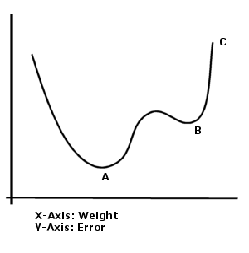
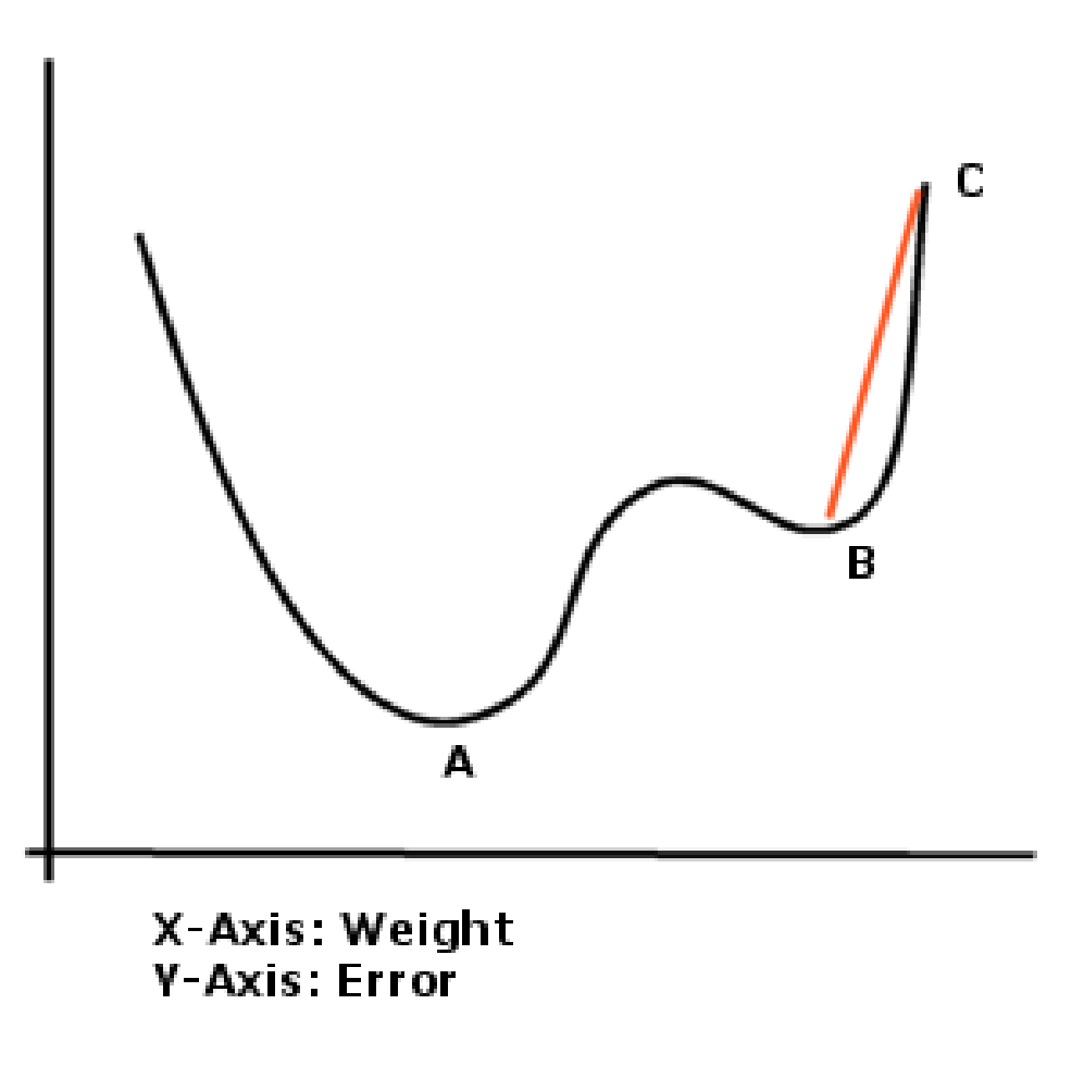
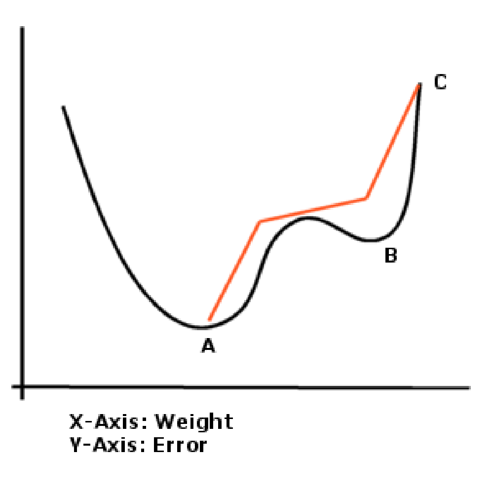
The principle factor with both of these training algorithms is the method in which they employ to minimise the difference between the obtained output of the network and that of the desired output of the network. In combination with the learning rate, the size of the error has a direct effect to how much each of the weights should be changed.
Because it is extremely unlikely that the neural network will be trained after presenting all the training patters once, it is necessary to keep presenting all the training patterns until either we have reached a limit where we decide the network will not be able to train any more (it may have reached local minima for instance) or the network has been trained enough so we can be confident that it can classify all of our inputs. Each time we one complete training cycle has been ended we say that an training 'epoch' has finished.
Weight adjustment can take two different forms. The first is batch mode and the second is incremental mode. Batch mode will find the error across the whole training set after each epoch of training and adjust the weights accordingly using this error. Incremental mode alters the weights after each pattern has been presented to the network.
Batch mode will be used in this project for simplicity as it is the default that MATLAB implements.
9.5.5 Training Method for the Feed forward Network
The training method used for the feed forward can be considered to consist of the following steps.
Initialise Weights
Do
For each training pattern
Train the network on current pattern
End For
Until output error is sufficiently small 68
Before a network can be trained the weights must be set to random initial values, this is done so that the activity of measuring the error between the desired output and the actual output can begin. If they were all set to zero the weights would have the effect of removing any of the input data into the network. The initial random weighting of the networks offers much discussion in the field of neural networks. Suffice to say that certain combinations of random weightings will mean the neural network can never be trained whilst other combinations can produce mediocre results or amazing results. MATLAB provides default functionality when choosing random initial weights, this functionality will be used when creating the neural network.
There is no need to develop the training function as this is already in place as part of the neural network toolbox provided in MATLAB. However, the "Train the network on current pattern", varies wildly from neural network to neural network. The neural networks that will be developed in response to this project will be trained using the gradient descent and gradient descent with momentum. Both of these are used with back propagation. Other training methods while they may be better are out of the scope of this project.
Training of the network will take place using selection ¼ of all the available data. The network will be tested using another ¼ of the data to see how well it performs. Finally, the network will be validated on the remaining ½ of the data to ensure that it can generalise for data that it should never have seen 69 . Data is not taken in sequential order, but from equally distributed points through out the data, this is standard practice as it can help to eliminate measuring the a customers aggregated account details twice and give rise to a better spread of sampling data.
Training using fixed parameters for the learning rate and the number of training sessions (epochs) alone is not sufficient to be able to successfully determine if this project has succeeded. Therefore, a variety of epochs ranging from 500 to 3500 will be used along with a sufficient number of variations of the learning rate. By adjusting the learning rate, we may achieve faster convergence on a solution, it may also enable us to miss local minima with respect to the error function. For the same reason, gradient descent with momentum is used (to try and avoid getting caught in local minima).
9.5.6 Problems Which can be Encounter when Training
When training the neural network we must be aware of two problems. The solution to these problems have already been defined, but the reasoning has not been justified.
When the network is training we can reach three conclusions: 70 71
- The network was not trained enough. It cannot classify enough of the training data for us to say it will be of any use to us when attempting to classify data it has never seen before.
- The network can be over trained. An over trained network may correctly classify all the data it has be trained on, but it will be too inflexible when it comes to classifying data that it has never encountered before.
- The network can classify most of the input correctly, but it has not been trained to such an extent that it cannot correctly classify data that it has never seen.
Obviously the third situation is the most suitable and obtained by varying the number of epochs that the network uses to train itself on the training data. We can then get a selection of neural networks from which we choose one which is the best.
9.5.7 Inputs defined in the NN.
When considering how to design the neural network it is important to understand the relation of the inputs to the neural network with respect to the output produced by the neural network. The adage "garbage in, garbage out" is pertinent, if the neural network through its training regime cannot discern any semblance of a pattern, the likelihood of the correct classification for the data is drastically reduced. This is the reason why research into the telecommunication industry was carried out, if none had taken place then more likely than not a neural network that classifies a customer's account correctly will not be created.
Once input data has been generated it must be processed. By reducing the number of inputs to the network, pre-processing helps the network to learn more effectively, as the likelihood of data correlation being identified is greatly increased. Two methods commonly used are transformation and normalisation.
Transformation can combine the generated data inputs into a single input; that is altering the input in such away that input still represents something close to what the pre-combined inputs meant. This implies that we can represent the same information with fewer input nodes. 72
Normalisation alters an input feature such as call duration so to distribute the data evenly across the data set and to scale the data to match the data range of the input neurons (so that the input data can be correctly scaled between -1 and 1 or 0 and 1 depending on activation function used and no matter what the data, it will always be in the range specified). 73
In most neural network applications, transformation involves statistical manipulation of the input data. For example, to understand the quantitive value of a customer call account, the types of information that is pertinent must be established, for instance a mean value of a customer's account attribute is not sufficient on its own, the standard deviation or variance must also be included, so that the nature of the average can be ascertained. For instance if the mean call duration is 20 minutes, we would want to know how spread of the call durations, as a smaller the spread could indicate that some automatic call device is being used.
Therefore the processed inputs may include items differences and ratios, rather than separate inputs. Each of the neurons in the network's input layer will represent one of the processed inputs.
Many transformation and normalisation methods exist, however some are more appropriate than others, for specific applications. Now that the basic network architecture has been decided upon (a MLP using back-propagation), it is important to establish what inputs must be used in the network. These inputs will be the final ones used, and thus it is important to establish why they have been chosen. If in the telecommunications industry, rather than using a model generation tool which will no matter how well developed never truly represent the client base. Analysis of the inputs to the network would be far more in-depth.
However, one must also consider the speed at which the data can be extracted from the database. It is no good extracting information about a customer from the database if it takes you 3 hours to get that piece of information.
9.5.8 Proposed inputs.
On initial inspection, it may seem logical to have every call type (PRS, free, local, national, mobile and international) available as an input to the neural network, with associated information, such as average call cost and average call duration, along with the spread of the data for each.
However, this method will mean that for our test situation approximately 30 inputs will be required (six call types each with at least four inputs). This is too many; too many inputs will mean that it is harder for the network to learn how to generalise, also some of the inputs maybe redundant having no effect on the output.
There are several ways to deal with this; one is by a process of elimination and combination (remove ones we know are not having an effect, or combine several inputs), the other method is via automated principle component analysis, which attempts to find components in the data that have high correlations.
I propose rather to have a simple segregation of the call types: high risk and low risk. This can greatly reduce the number of inputs that the network requires to use.
High Risk calls are international calls, mobile calls and PRS calls, whilst low risk calls can be considered to be Local, National and free phone numbers. All inputs to the neural network are shown in table 4.
Table 4 Input Parameters to the neural network
|
Input |
Description |
|
Number of Low Risk Calls |
The number of low risk calls made during the period of analysis. |
|
Number of High Risk Calls |
The number of high risk calls made during the period of analysis. |
|
Incoming calls in the period |
The number of calls made during the period can be used as an indicator of fraud. If the customer makes a plethora of calls whilst receiving a relatively small proportion of call (in comparison to the number of calls made) then the customer might be running some sort of call selling scheme. |
|
High risk ratio |
A ratio of high risk calls as a proportion of all the calls made, can be indicative of a fraud occurring. |
|
Low risk ratio |
A high ratio of low risk calls in proportion to all the calls made could indicate that the customer might not be acting fraudulent, with regard to scams such as call selling. |
|
Low risk average cost per call |
Used to establish the average cost of a customers calls that have been graded as low risk. This is present to counterbalance the high risk average call cost feature from consuming the neural networks decision to distinguish between fraud and non-fraud customers. |
|
High risk average cost per call |
If the average cost for all the calls is high then, it could indicate that some sort of fraud is occurring such as call selling or PRS fraud, combining this with a high ratio of high risk calls could be a further indication of fraud taking place as a lot of money is being spent on calls. |
|
Low risk cost per call standard deviation |
This like many of the other features of the network, is to balance out the effect of the high risk features. |
|
High risk cost per call standard deviation |
If the standard deviation of the high risk call costs is small, it may be indicative of a fraud scheme such as those committed by PRS fraudsters. They might be using a some sort of automated dialler. |
|
Low risk average call duration |
Used to establish the average duration of calls that have been classified as low risk. This is present to counteract the high risk average call duration feature from overpowering the neural networks decision to distinguish between fraud and non-fraud customers. |
|
High risk average call duration |
A high average call duration on high risk calls might be indicative of a customer making long duration calls to PRS or International numbers. This might therefore be indicative of fraud. |
|
Low risk call duration standard deviation |
This like many of the other features of the network, is to balance out the effect of the high risk features. |
|
High risk call duration standard deviation |
A low standard deviation of call durations, might indicate an automated call dialler scheme is in operation, since these may operate using fixed redialling machines that will stay connected for a set period of time. |
You may ask, why are both high risk and low risk properties of a customers account being considered as inputs to the neural network?
Take for example a company who may operate both nationally and internationally. A proportion of the calls will be high risk and likewise some calls will be low risk. If we only considered the high risk calls, then the customer may appear to be fraudulent and the neural network may not be able to pickup on this relationship (there is no relationship since high call durations to international numbers could either be fraudulent or not).
Therefore, if we have the ratios and properties of low risk calls as inputs, the network should be able to establish that many high-risk calls in the presence of relatively few low risk calls could be deemed more fraudulent than lots of high risk calls I the presence of plenty of low risk calls.
Each of the inputs will be bi-polar, thus will be normalised between -1 and 1. This has the effect of resolving the issues of having one of the network inputs as a zero, which can effectively turn off a node. If an input is zero, the node receives the input multiplied by the weight, which will still be zero; it may be that this feature is an important and the network will now not take any notice of it. Therefore, if the input is -1, the network can operate on this feature and still understand that it is distinctive of one class of data.
9.5.9 Consideration of the Data Being Presented to the Network
The data that is being presented to the neural network is aggregated over two week periods (as mentioned in section 9.3.4.6).
To ensure that enough data is being trained on, two months worth of data is being generated by the call generation tool. Therefore, for each customer four windows onto the data are being presented to the network, each starting and ending at the two week boundaries.
More information from each customer could be provided if the sliding windows algorithm were to be used (increment the start of the window by one day). However, the nature of the call generator will mean that though the data generated is random, and even if the windows on to the data were moved, the customers calling patterns should still be the similar, as their day to day activity over a two week period will not vary to a large degree. To keep things simple and efficient the windows onto the data are simply spaced on the two week boundaries. This also will help with the training as only one pattern for each customer is trained on, implying that the network will not be trained on any one customer more than any other, this should help with the generalisation ability of the network as it has been given the broadest representation of customers available.
9.5.10 Consideration of the Output of the Network.
The output of the network is probably one of the most important parts of the neural network. If the output is wrong or is ambiguous then the results obtained will mean that any FMS based on this idea of a neural network will not work.
When training the network the output of the network will be compared against a 1 for a non-fraudulent account and a -1 for a fraudulent account. This decision has been taken for several reasons; the first being that the activation function on the other nodes in the network are bi-polar, it stands to reason that keeping things even will be better; the second is that MS Access stores a 'FALSE' value in a Boolean field as -1, so to save having to transform every network output keeping the output at -1 is recommended.
When running data through a completed network, the output will therefore be in the bounds of -1 and 1, but it will never be actually able to give the output of -1 and 1 due to the nature of the tan sigmoid function (the results will get infinitesimally close to the two limits but never reach them). The closer the data is to any of the bounds then the more confident the neural network is that the input which was supplied is of a certain class.
The network will also require a threshold function which will say above this value the customer account for the specified period has been deemed to be non fraudulent, otherwise it is fraudulent.
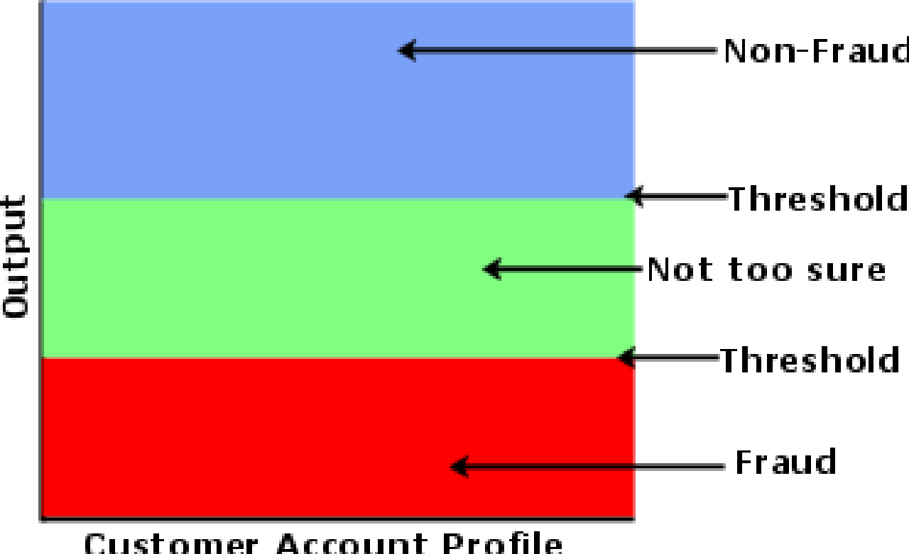
Figure 30 Dual Threshold System
There are two schools of thought when using a threshold function for the output; you can use two thresholds or one. The two threshold method will state for threshold 1, anything above the value is clear; the second will say anything beneath my value is fraud; finally anything lying in the middle ground will be considered fuzzy (i.e. not too sure).
Figure 29 Single Threshold system
The single threshold system has been chosen because if a customer account appears in the "not too sure" region in the two threshold scheme, it would be wise to still investigate the customers account further. Therefore, the distinction between the two methods has been diminished as all fraudulent accounts always have to be investigated before a fraud analyst can take further action to prevent the customers access to the telecomm network. Therefore, all accounts which they are not too sure about will also have to be investigated. The fraud analysts might as well have them classified as fraud in the first place.

The output of the network will only use one node for simplicities sake, however more can be used, depending on the number of output classes needed. This project only requires one output because the data can be split into two separate classes (clear and fraudulent, clear being signified as 1 and fraud as a -1). However, we could have had two output nodes, one for each class.
9.6 Neural Network Creation Tools Design
Several tools have to be designed to facilitate network training, data extraction and performance analysis. It is important to create software that will perform the functions, because even though they can be easily created by hand with MATLAB, analysis of the performance and the relevance of the networks cannot take place
9.6.1 Training Tool
The focus of the training tool is to generate a large set of networks that can later be analysed. The reason why a large set of neural networks need to be created is, because depending on the initial weights when training the network many never converge on an optimal solution; it may never converge on any sort of solution at all. Before any form of neural network can be recommended as an appropriate solution, it must be shown that the one being presented is the best one available, as if other networks could perform better why are they not being shown as the optimal solution.
Training takes place by varying the number of nodes in the hidden layer. This ranges from 5-10 hidden nodes. Each network of the different number of hidden nodes must each be trained in similar fashion. The manner in which each of these different types of networks are trained can be described as follows:
- The number of epochs must be altered, as to ascertain if extra training does affect the overall performance.
- The learning rate must be altered. To small a learning rate might cause the network to get caught in locally optimal solutions or may mean that the network will take too long to converge on a solution, while learning rates which are too large may never be able to converge on a solution at all as the changes in the weights might be too large instead the weights would oscillate around the minimum solution but never actually achieve the desired result.
- Different data combinations must be trained on, since if we did not randomly choose the data the network was to train on the network might not have a diverse enough range of inputs to learn from, so that its future ability to generalise answers to unseen inputs would be severely diminished.
The algorithm used is depicted in the figure 31 and is the same algorithm for both the normal gradient descent method and gradient descent with momentum all that is changed is the training function which MATLAB uses to train the network.
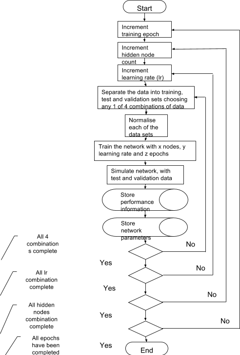
Figure 31 Training Tool Data Flow
9.6.2 Data Extraction
Figure 32 Data extraction tool data flow
The data extraction process is a simple piece of the development. Without the data extraction method, there would little or no way to get the data out of the Microsoft Access 2000 database. Essentially, all that happens is MATLAB connects to the database via an ODBC connection specified as a 'User DSN'. Once connected the SQL statement is passed through the connection. Following this, the results are then 'fetched' from the database and stored in a MATLAB variable.
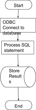
There are two main types of data extraction queries. The first query simply returns the information about each customer in bi-weekly summaries. The second methods is then issued to ascertain if each of these summaries is either fraudulent or clear.
9.6.3 Performance Analysis and Testing
The performance analysis takes the form of throwing away the networks that could never classify any of their data and then establishing which of the remaining neural networks performed the best.
The performance of a neural network can be measured using the mean squared error (MSE) on the output of the network once it has been trained. The MSE represents the average error (difference between the expected output and the actual output) on the output for all of the input patterns presented to the network. Although this might seem to be a good indicator of performance; alone it is not. The network might have been trained too much on one subset of the data; therefore, its ability to classify unknown and unseen data would be severely reduced. It is also hard to visualise what the output of the MSE signifies in relation to how many completely erroneous results occurred (for instance 10 customers might be incorrectly classified, but the MSE could still be low, if the rest of the customers are classified with little error). This is where the Receiver Operating Characteristic (ROC) curve comes in. The ROC curve can give us a visual representation of how well a neural network will work by showing misclassification rates.
The first step of the performance analysis is to generate a ROC chart for the data that the neural network has been trained on. The ROC chart can be used to analyse the ratios of false negatives, false positives, true positives and true negatives. The area under the ROC curve is considered a good indicator of how well classification has been performed.
For this project, the following guidelines for case classification have been setup. A non-fraudulent account is considered as a positive (because this is how it comes out of the database), many systems consider a fraudulent account as positive, but both methods are interchangeable.
|
True Positive |
A correctly classified non-fraudulent customer account. |
|
False Positive |
An incorrectly classified non-fraudulent account |
|
True Negative |
A correctly classified fraudulent customer account. |
|
True Positive |
An incorrectly classified fraudulent account |
If we measure the performance with consideration of the non-fraudulent customers in mind, we can establish the levels at which we can get 100% classification of non-fraudsters and roughly what percentage of fraudster will be classified as non-fraud (if we want every customer who is not fraudulent to be classified so). This is important since totally missing the fraudsters will mean lost revenue, saying a customer is fraudulent when they are not (although important) may not lose the company as much money.
A ROC chart is generated by plotting all sensitivity values (true positive fraction) on the y-axis against their corresponding (1 - specificity) values (false positive fraction) for all available thresholds on the x-axis. 74 75
Y-Axis (Sensitivity):

Figure 33 Y-Axis for ROC Chart (Sensitivity)
X-Axis (1-Specifity)

Figure 34 X-Axis for ROC Chart (1 - Specifity )
For each threshold value in the network (ranging for -1 to 1), the sensitivity and the 1- specificity are calculated and plotted. In the final network we therefore locate the point where the network has the highest number of correctly classified results is obtained.
The area under the ROC curve is used as an indicator as it can provide an overall score to how well the neural network performed no matter where the threshold value is located. The larger the area of the ROC chart means that there is less overlap between the two classes (one class being judged as another class/non-fraudulent accounts being classified as fraudulent), an area of 0.5 means that the tool being used to judge which class the input is in, cannot distinguish between either of the two classes of data.
The area under the graph can be determined using the trapezoidal rule. 76
By only considering the networks which have an area under the ROC chart of more than 0.6 we can remove the networks that will never be able to classify any results. The results of one such network, which could not classify the result correctly, can be seen in figure 35. (An area of less 0.6 will mean that there is a high overlap of results and that only 60% of the time a non-fraudulent customer will have a score from the neural network above the threshold for deciding if the customer is clear or not).
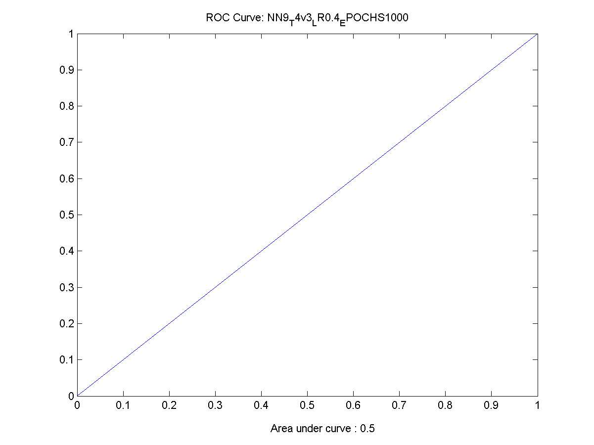
Figure 35 An incorrectly trained neural network ROC depiction
As can be seen in figure 35, the area is less than 0.6 and when looking at the results, and essentially the graph is indicating there was no classification of accounts where all the fraudulent accounts were not included in the non fraudulent set of accounts, however there were no non-fraudulent customers classified as fraudulent. If this was the case the curve of the graph would be bowed and look something like an exponential curve.
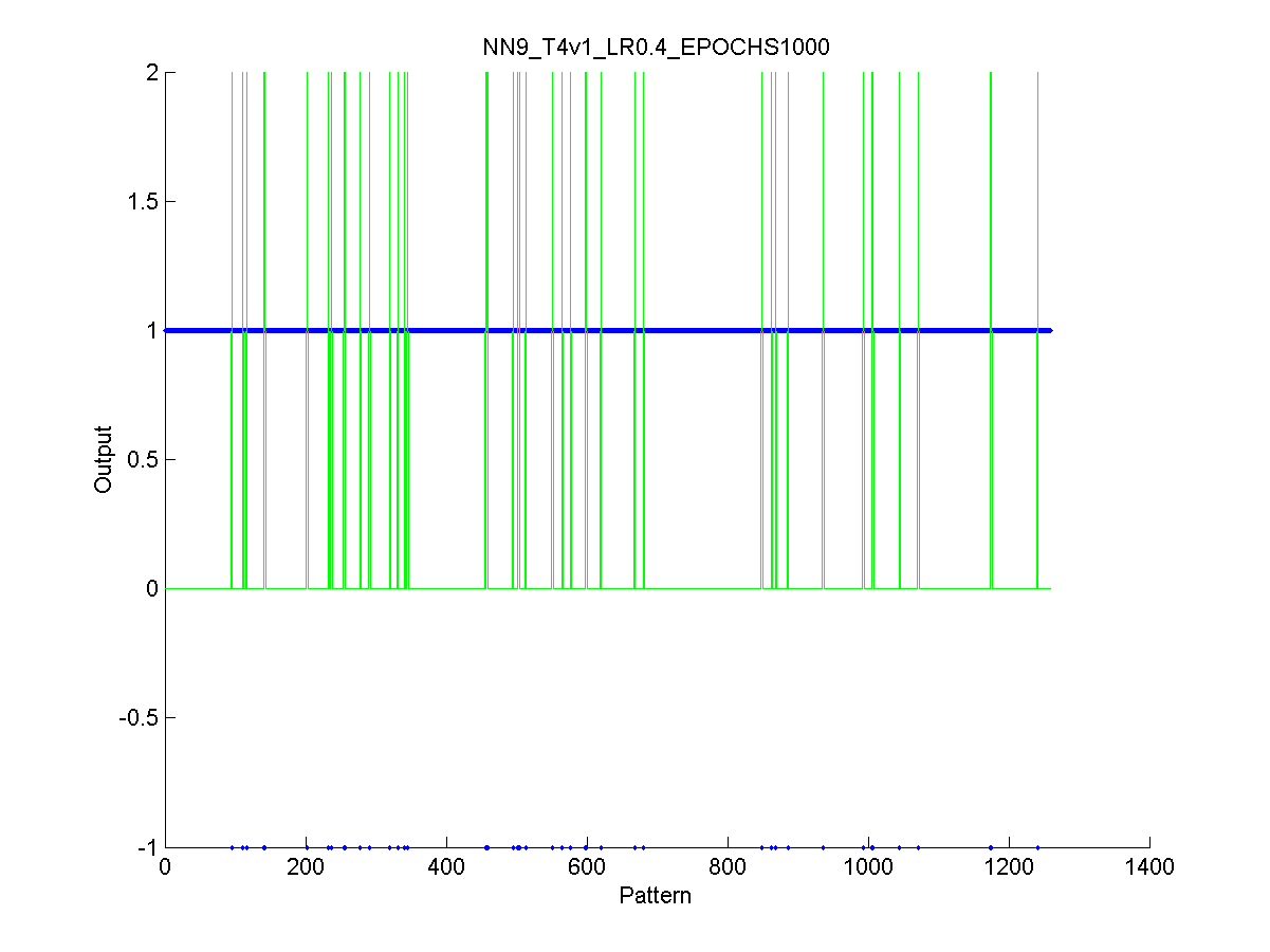
Figure 36 Actual output of an incorrectly trained network
Figure 36 is further proof that not a single fraudster was classified correctly (a value of 1 being clear and -1 being fraudster).
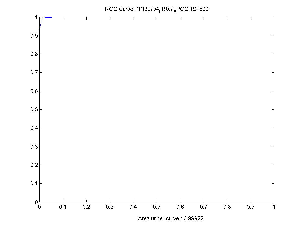
Figure 37 ROC Chart for a working neural network
The next ROC chart (figure 37) shows a network whose performance was extremely good. The networks can correctly classify approximately 90% of the non-fraudulent customer accounts, without classifying a single one of the fraudulent accounts as non-fraudulent.
However, according to the figure 37, if we want to correctly classify 100% of the non-fraudulent accounts we must accept that about 8% of the fraudsters will be classed as clear. That is to say 8% of all the fraudsters would manage to slip through the net if we wanted to ensure that not a single person was falsely accused of fraud.
The second stage of the performance analysis is to establish how well the network performs on a totally new data set. This method is used to establish if the neural network can work with data that it has not been trained on. If it can, then we will see very little difference between the two areas underneath each of the ROC charts generated on the separate sets of data. If not then there should be a decrease in the area under the second chart, implying that the networks performance also decreased.
Initially we remove any of the networks where the area under the ROC chart for the first set of data is less than 0.6, which indicates that the network may have classified one of the two output classes (Fraud or Non-fraud) 100% incorrectly. We then compare the results of each of the neural networks against both data sets. The complete process can be seen in figure 38.
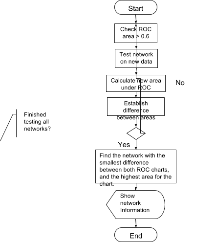
Figure 38 Data flow for establish the performance of the neural networks
9.6.4 Establishing the Most Appropriate Threshold for the Final Network.
Now that the final network has been established, a value for the threshold must be given; the threshold is the value where all the call patterns whose neural network output is greater than the threshold will be considered not to be fraudulent, while the output of the network which lie beneath the threshold will be classified as fraudulent.
This value will be ascertained by hand because it is assumed that if the network works well then there will be a visible distinction between the boundaries of both classes.
9.6.4 Testing the Network Creation Tool.
The principles that are being used to test the CDR generation tool (section 9.3.4.8) will be applied to the tools used to create the neural networks. That is black box testing will take place on the functions. Because I am not making a full program in the prototype, I only see the need to create functions that will help me speed up my analysis of the results. Essentially, what is being created is a set of Macros in MATLAB and the testing will provide proof that the functions work as specified.
Test plans and results are supplied in the appendix (16.4.2)
9.7 Models Generation
The models used to generate the call data are important aspects of the system. If they are incorrect then we cannot prove they will help the fraud analysts to detect fraud. Having too few call models may mean that they neural network was able to model the problem too easily, but having too many may mean that the neural network is unable to establish the features associated with each customer class. This is an important fact to consider as there are more call classes and customer belonging to a telecoms company than I can generate or research myself.
9.7.1 Methods to generate the best models.
There are several issues that need to be dealt with when designing the models. These issues can be summarised as follows:
- I am unable to obtain real call data that is generated by telecom companies;
- The classes of customer are unknown, the best that can be done is to think of the types of people there are using the system;
- The call patterns for the classes is also unknown, so the best that can be hoped for is to mimic call patterns after some research.
The best method I could find to generate the customer classes is to look at the phone bills of friends and family and also of companies that I am associated with. Even though this will only account for a small cross-section of the customer accounts on a telecomm system, I can use the data I have gathered first to model how the group the participant would appear in acts. Additionally, extrapolate from this and say something along the lines of "okay this is how company X operates who are a small company with 5 people in, therefore, a medium sized company with 30 employees might have 9 times as many call, with more being international". Obviously, this method is not the most accurate way to model customer classes and is very flawed, but it is the best bet for this project.
There were two stages of model creation; the first ran into problems because there was little overlap between model groups and the neural network classified them too well. This effectively meant the models generated were not like what might be seen in real world telecom fraud analysis. This problem will be discussed further in the evaluation of the results.
The quantity of data being presented to the networks is also important. If we trained the network only on fraudulent accounts it would not be able to classify clear accounts and vice versa. If the number of fraudulent accounts presented to the network is more that the proportions of fraudsters we seen the wild, then this prototype tool would be useless because it would be too sensitive to fraudulent information and would more than likely classify non-fraudulent people as fraudulent.
Determining the proportions of fraud is an important step, as mentioned in section 7.4.2 approximately 3% of telecoms revenue are lost due to fraud. We could therefore say that 3% of the customers are fraudulent and therefore if we had 1000 customer accounts about 30 of them would be fraudulent. This is a rough estimate since if a person is trying to defraud a telecomm company are they only going to make a few calls? more likely they are going hit the telecom company for all they can. Therefore the number of fraudsters is probably less in proportion to the revenue lost by all fraud. However telecommunication companies do not publish this information, so sticking with roughly 3% of all customers are fraudulent is a good idea.
The second set of models (which are the ones used in the final tests) allow for overlap between fraudulent and non-fraudulent customers. The models and reasons for selection will be discussed next.
9.7.2 Brief discussion about the models used.
A more in-depth discussion of the models can be found in the appendix (section 16.5), but what follows in table 5 is an outline of all the models used.
Table 5 Models used in the creation of the customer data
|
Model Name |
Model Description |
N o of Accounts |
|
Normal Average |
A normal customer making normal use of the network |
200 |
|
Normal No International |
A normal customer who makes no international calls whatsoever. |
200 |
|
FRAUD - CALL SELLING International |
An International Call selling operation |
6 |
|
FRAUD - PRS |
A PRS scam which makes many of short duration calls all of a similar period |
12 |
|
FRAUD - PRS 2 |
A PRS scam which makes lots of long duration |
10 |
|
Business - Shop |
A small shop – has one possibly two phone lines |
100 |
|
Business - Small |
A small business – has about 5 phone lines |
50 |
|
Business - Medium |
A medium business – has about 10 phone lines |
40 |
|
Business - Large |
A large business – has many phone lines |
20 |
|
Home - Internet Access |
A home user who makes long duration calls on the internet, and automatically redials when cut off. |
200 |
|
Home - Plenty Of International |
A home user who makes lots of international calls for a relatively long period of time |
200 |
|
Fraud Home Call Sell PRS Hidden |
PRS scam, which is hidden inside what appears to be a normal customer account |
10 |
The ratio of fraudulent customers to clear customers can be shown to be:
1010 clear customers; 38 fraudulent = 3.8% of customers are fraudulent.
The above models represent as best that can be with the model generator classes that are not easily separable from each other, this can be seen by such accounts as the Fraud Home Call Sell PRS Hidden where PRS fraud is hidden with he guise of a normal customer. Another example is a normal customer ( Home - Plenty Of International) who might have the properties of a call seller , this could be a customer who wants to call relatives abroad.
The neural network must be trained to a level where it can understand the ambiguity in the customer information.
10. Analysis of Results
What follows is the analysis of the results from the neural networks. Each individual network that was created will not be discussed, but rather the final networks which have been to perform the best.
Each network class (number of nodes in the hidden layer) will be combined into a super group of neural network. A new set of data will then be presented to each network in this super group; this data has never been seen before and will differ from the data that each of the networks has been trained on.
This data will be generated using the same model parameters, but because of the method in which the random data is generated, no two customer call patterns will be the same and therefore reinforce the notion that neural networks can generalise a solution from data that they have never been aware of before.
The final network that will be chosen will be the network that has performed the best across both sets of data. Along with a small conclusion as to why I think this network outperformed the rest of the networks.
Neural networks with an area of less than 0.6 will be discarded and not considered, this is because they have not been able to ascertain when a fraudulent account is fraudulent.
10.1 Overview of how to study the graphs
When each network has been produced, various performance functions are used to measure how good the network was at classifying the results. The performance functions of this project with respect to the networks are fourfold. It is important to understand these graphs as they are presented on a CD in the appendix as there are too many to reproduce in this project.
- The performance function of the training set after each epoch.
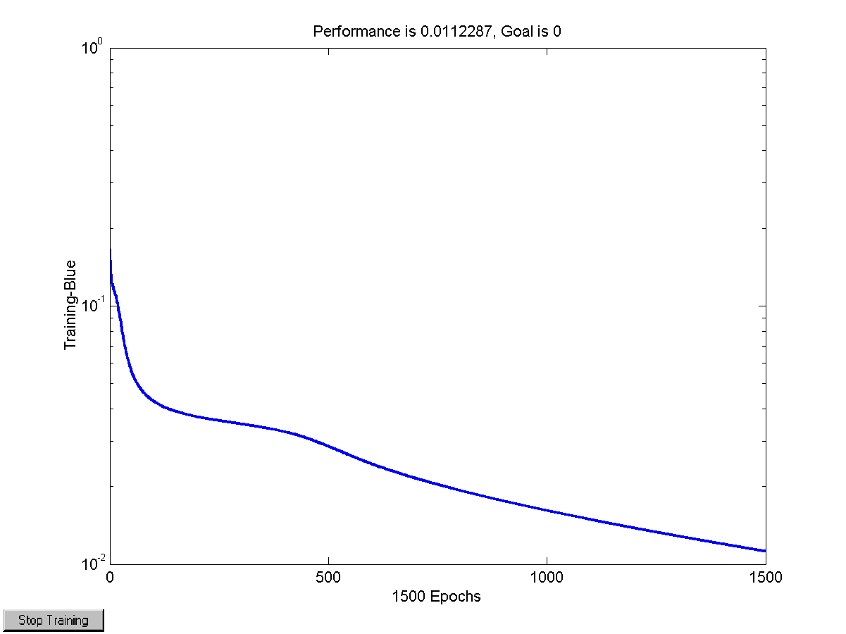
Figure 39 Performance of the training algorithm
The graph is based on a semi-logarithmic scale and represents how the error has been reduced through the training of the network. After each epoch the 'mean squared error' is established and plotted. Here we can see that after the 1500 training sessions the mean squared error (or the performance) was 0.0112287. This graph was produced using a 7 hidden node network, trained with a learning rate of 0.1 and had 1500 training cycles using normal gradient descent as the error reduction function. As can be seen, initially the rate of change in the error was high; it then petered off until and remained pretty constant for the remainder of the training set.
- The output of the network in relation to the expected output of the network after the test stage.
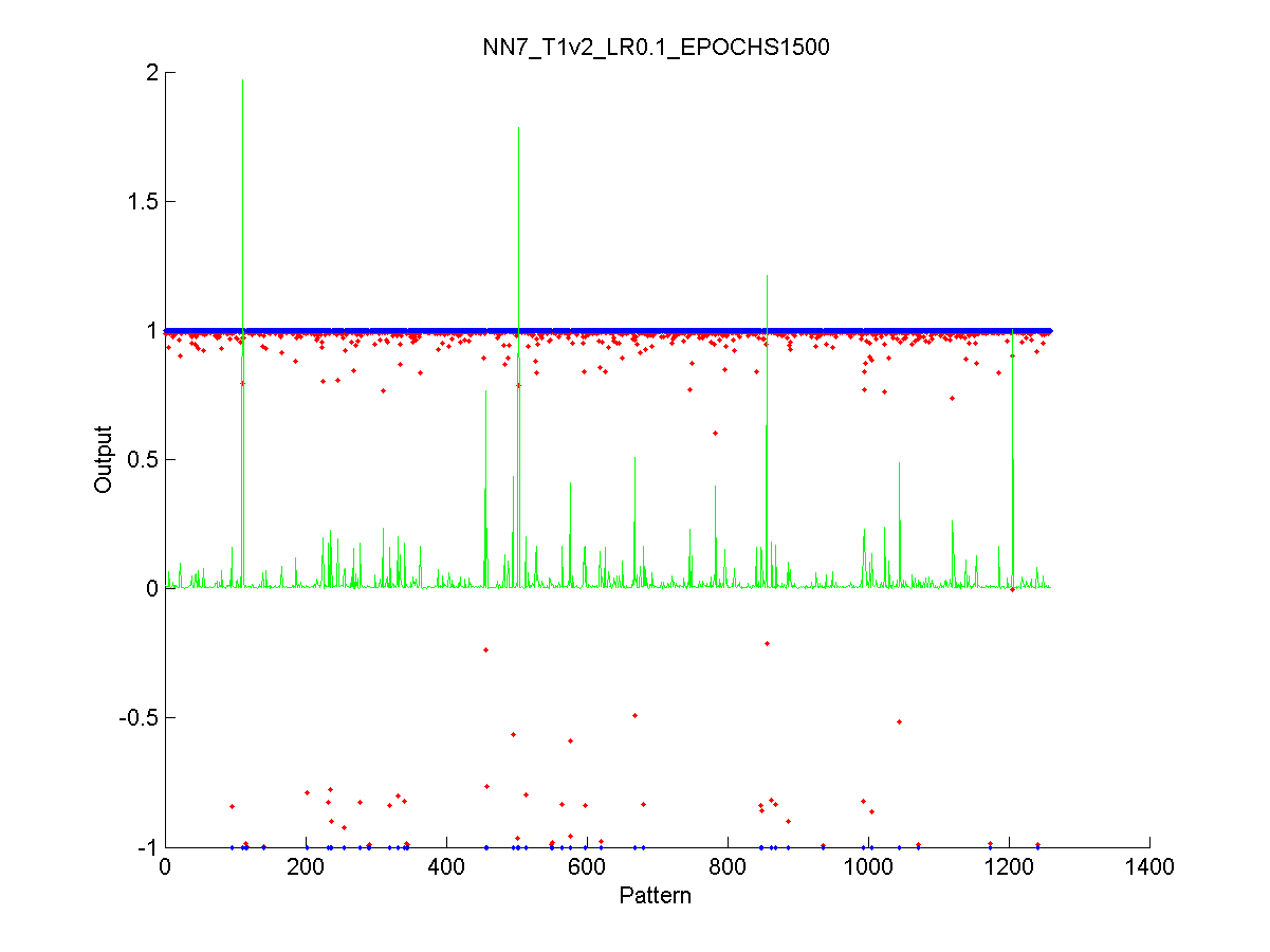
Figure 40 Output of the neural network after the test stage
This graph shows that the network was trained using approximately 1200 different customer profile patterns.
The blue dots represent the desired output of the network and can be clearly seen at the extremes of the output. The red dots represent the output that the network produced (which can be seen in black and white as the points not at the extremes) , while the green line represents the difference between the desired output and the actual output.
Although some of the predicted output is far away from the expected output; accurate location of the threshold value will still mean that they are correctly classified, however as the magnitude of the error nears to two it signifies that this particular pattern will almost certainly never be classified correctly.
- The output of the network in relation to the expected output of the network after the validation stage.
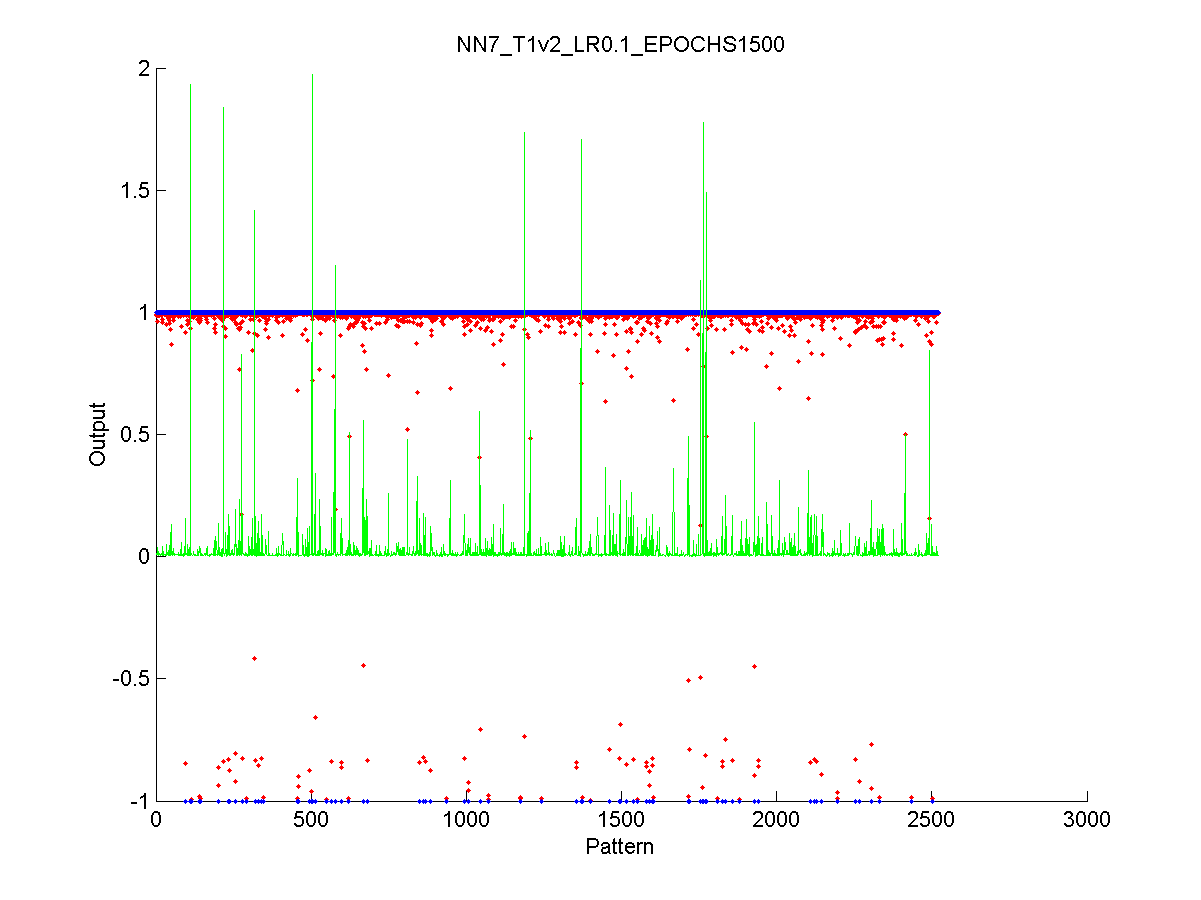
Figure 41 Output of the neural network after the validation stage
The above graph is based on the same principle as the training test. However, this time it is ran on the remaining set of the data, which the network has never seen. It is simply used to visually classify the performance of the neural network. The more green lines that are present which near the magnitude of two then the likelihood that the network will not be able to classify the customer correctly, as this is the data that has never been seen by the network before.
This graph is also a good indicator of future performance of the network as the data presented has not been seen before, so if it can classify these well then it is likely that it will be able to classify other unseen data just good.
The ROC is a better classifier of performance.
- The ROC graph showing the classification level of the network, the number of true positives and true negatives (sensitivity) against the number of false positives and false negatives. Essentially this is the misclassification rate.
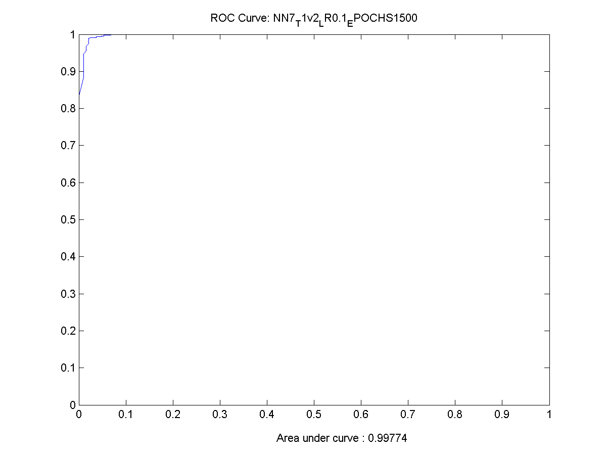
Figure 42 ROC Chart
The above graph represent the a network with 7 hidden nodes trained on the second available data set with a learning rate of 0.1 and had 1500 training cycles using normal gradient descent as the error reduction function.
What we can see is that given any threshold value (above and including which accounts are considered clear and beneath which they are deemed to be fraudulent) we can expect roughly 80% correct classification of non-fraudulent cases without having a fully misclassified fraudulent customer account. However, if we want to get 100% correct classification of True positive events (non-fraudulent customers), then we have to have to accept that 10% of the cases presented as non-fraudulent will be misclassified (False Positives) fraudsters (i.e. they have slipped though the net).
All 17,000 performance graphs are available on the CD supplied in the appendix.
For a network to be considered as the final network the difference between the area under the two ROC graphs should be minimal. The performance is quantified in the following manner:
- Establish the maximum difference of the size of the areas between nodes that have not been discarded. This is then 100% difference.
- Every network is then classified as a percentage of the maximum distance.
- The networks with the lowest percentage area difference are considered.
- The network with the largest area is put forward to be final network.
To find the final neural network, I could simply find the network which has the highest are under the ROC curve and the smallest difference between the two sets of data, however to be more through a more in-depth analysis of each of the groupings of nodes will take place. The final network will be represented by the best performing network out of all of the networks generated, but also with a description to why it has been chosen.
Number of training failures taken into account for each different size network (the number of hidden nodes). The more failures when training means we are more likely not to get a satisfactorily trained network using that particular network architecture.
10.2 5 Hidden Nodes

Figure 43 MATLAB depiction of a 2 Layer network with 5 nodes in the hidden layer
A hidden layer with 5 nodes, on average after training, the network had the following performance classification based on the area under the ROC chart.
Table 6
|
Difference Percentage |
Networks in this group |
Percentage total of fully trained networks |
|
0-10 |
266 |
95% |
|
10-20 |
10 |
4% |
|
20-30 |
3 |
1% |
|
30-40 |
0 |
0% |
|
40-50 |
0 |
0% |
|
50+ |
1 |
0% |
432 Networks in total with 299 fully trained networks
280/432 * 100 = 64.81% successfully trained networks
Network proposed as final network from this group:
Internal Name: NN5_T4v2_LR0.4_EPOCHS3500
This network was trained using a learning rate of 0.4 with 3500 training epochs.
The area under each of the ROC graphs
Area under ROC1: 0.9994
Area under ROC2: 0.9994
The performance of these networks are good, nearly 65% managed to be trained. The highest performing network could classify 100% of the data patterns presented to it, however better performing networks were present. As can be seen in table 6 a lot of the networks had very similar performance and the areas under the ROC curves did not differ much for the majority of the networks.
10.3 6 Hidden Nodes

Figure 44 MATLAB depiction of a 2 Layer network with 6 nodes in the hidden layer
The networks with a hidden layer with of 6 nodes, on average after training had the following performance classification based on the area under the ROC chart.
Table 7
|
Difference Percentage |
Networks in this group |
Percentage total of fully trained networks |
|
0-10 |
183 |
73% |
|
10-20 |
7 |
3% |
|
20-30 |
37 |
15% |
|
30-40 |
8 |
3% |
|
40-50 |
5 |
2% |
|
50+ |
11 |
4% |
432 Networks in total with 251 fully trained networks
251/432 * 100 = 58.11% successfully trained networks
Network proposed as final network from this group:
Internal Name: NN6_T5v2_LR0.5_EPOCHS3000
This network was trained using a learning rate of 0.5 with 3000 training epochs.
Area under ROC1: 0.9993
Area under ROC2: 0.9993
The performance of these networks are good, nearly 58% of the networks were successfully trained. The highest performing network could classify 100% of the data patterns presented to it, however better performing networks were present. As can be seen in table 7 a lot of the networks had very similar performance and the areas under the ROC curves did not differ much for the majority of the networks, however more networks in this node group differed from each other than in any of the other network groups, suggesting that the training performance for these networks was erratic or that some networks had been over trained.
10.4 7 Hidden Nodes
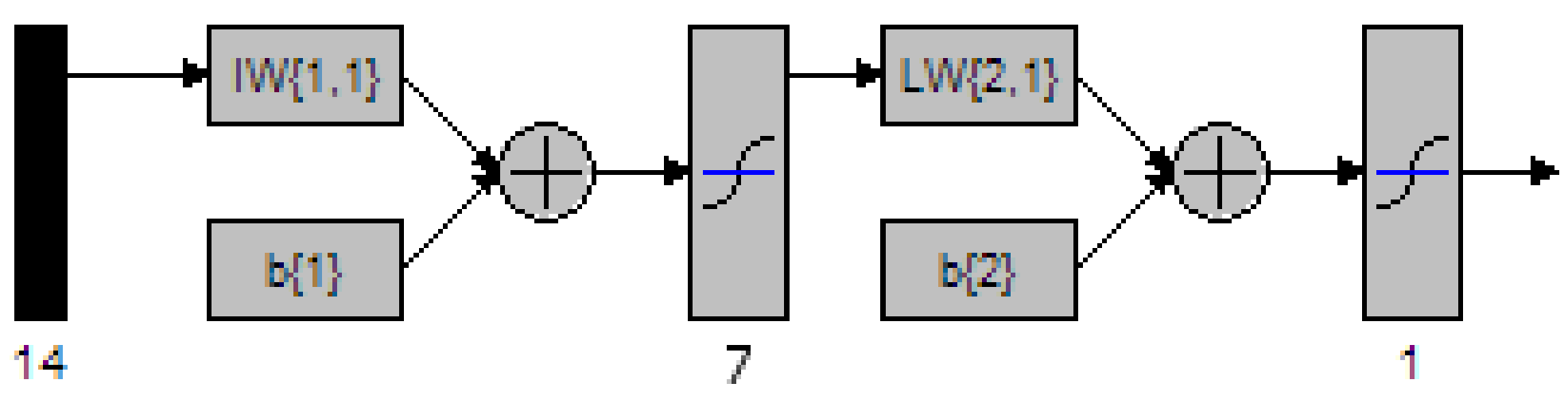
Figure 45 MATLAB depiction of a 2 Layer network with 7 nodes in the hidden layer
The networks with a hidden layer with of 7 nodes, on average after training had the following performance classification based on the area under the ROC chart.
Table 8
|
Difference Percentage |
Networks in this group |
Percentage total of fully trained networks |
|
0-10 |
187 |
81% |
|
10-20 |
33 |
14% |
|
20-30 |
4 |
2% |
|
30-40 |
4 |
2% |
|
40-50 |
1 |
0% |
|
50+ |
3 |
1% |
432 Networks in total with 232 fully trained networks
232/432 * 100 = 53.07% successfully trained networks
Network proposed as final network.
Internal Name: NN7_T6v4_LR0.6_EPOCHS3500
Area under ROC1= 1
Area under ROC2= 1
The highest performing network could classify 100% of the data patterns presented to it.
The performance of these networks are good, 53% of the networks were successfully trained with 81% of the networks performance deviating little between both datasets. As can be seen in table 8 a lot of the networks had very similar performance and the areas under the ROC curves did not differ much for the majority of the networks, a fair few of the networks performance differed quite a bit again suggesting that possibly some training anomalies arose and perhaps some networks were over trained.
10.5 8 Hidden Nodes

Figure 46 MATLAB depiction of a 2 Layer network with 8 nodes in the hidden layer
The networks with a hidden layer with of 8 nodes, on average after training had the following performance classification based on the area under the ROC chart.
Table 9
|
Difference Percentage |
Networks in this group |
Percentage total of fully trained networks |
|
0-10 |
238 |
95.58% |
|
10-20 |
7 |
2.81% |
|
20-30 |
1 |
0.40% |
|
30-40 |
0 |
0.00% |
|
40-50 |
0 |
0.00% |
|
50+ |
3 |
1.20% |
432 Networks in total with 299 fully trained networks
249/432 * 100 = 57.63% successfully trained networks
Network proposed as final network:
Internal Name NN8MOMENTUM_T5v1_LR0.5_EPOCHS1500
Area under ROC1 = 0.9994
Area under ROC2 = 0.9994
The performance of these networks are good, nearly 57% of the networks were successfully trained. The highest performing network could classify 100% of the data patterns presented to it, however better performing networks were present. As can be seen in table 9 a lot of the networks had very similar performance and the areas under the ROC curves did not differ much for the majority of the networks. The network trained on gradient descent with momentum performed the best this time and as can be seen needed only 1500 epochs to be trained, compare this to the networks trained using normal gradient descent which to get good performance needed in the range of 2500 – 3500 training epochs.
10.6 9 Hidden Nodes

Figure 47 MATLAB depiction of a 2 Layer network with 9 nodes in the hidden layer
The networks with a hidden layer with of 9 nodes, on average after training had the following performance classification based on the area under the ROC chart.
Table 10
|
Difference Percentage |
Networks in this group |
Percentage total of fully trained networks |
|
0-10 |
213 |
94% |
|
10-20 |
6 |
3% |
|
20-30 |
3 |
1% |
|
30-40 |
0 |
0% |
|
40-50 |
0 |
0% |
|
50+ |
4 |
2% |
432 Networks in total with 299 fully trained networks
226/432 * 100 = 52.31% successfully trained networks
Network proposed as final network:
NN9_T6v2_LR0.6_EPOCHS2500
Area under ROC1 = 0.9995
Area under ROC2 = 0.9995
The performance of these networks are good, nearly 52% of the networks were successfully trained. The highest performing network could classify 100% of the data patterns presented to it when given a threshold, however better performing networks were present. As can be seen in table 10 a lot of the networks had very similar performance and the areas under the ROC curves did not differ much for the majority of the networks. The network trained on gradient descent with momentum performed the best this time and as can be seen needed only 1500 epochs to be trained, compare this to the networks trained using normal gradient descent which to get good performance needed in the range of 2500 – 3500 training epochs.
10.7 10 Hidden Nodes

Figure 48 MATLAB depiction of a 2 Layer network with 10 nodes in the hidden layer
The networks with a hidden layer with of 10 nodes, on average after training had the following performance classification based on the area under the ROC chart.
Table 11 Results for the 10 node network
|
Difference Percentage |
Networks in this group |
Percentage total of fully trained networks |
|
0-10 |
205 |
95.35% |
|
10-20 |
6 |
2.79% |
|
20-30 |
0 |
0.00% |
|
30-40 |
1 |
0.47% |
|
40-50 |
0 |
0.00% |
|
50+ |
3 |
1.40% |
432 Networks in total with 299 fully trained networks
215/432 * 100 = 56.94% successfully trained networks
Network proposed as final network.
NN10MOMENTUM_T1v1_LR0.1_EPOCHS3500
Area under ROC1 = 0.9994
Area under ROC2 = 0.9994
93% of the 251 networks that were successfully trained and overall varied little in comparison to the rest of the other networks groups. The best performing network was trained using gradient descent, but still needed a lot of training; this is contrary to what I initially expected where I thought that networks with gradient descent and momentum would have required significantly less training to reach the same performance levels as the networks trained just on gradient descent alone.
10.8 Final Node
The final network; the network that I propose to use for the system has the following properties:
Name: NN7_T6v4_LR0.6_EPOCHS3500
Inputs: 14
Hidden Neurons: 7
Output Nodes: 1
Learning rate: 0.6
Training data set: 4
Epochs: 3500
Training Algorithm: Gradient Descent
The reasons for this choice of this network are as follows:
Area under ROC1= 1
Area under ROC2= 1
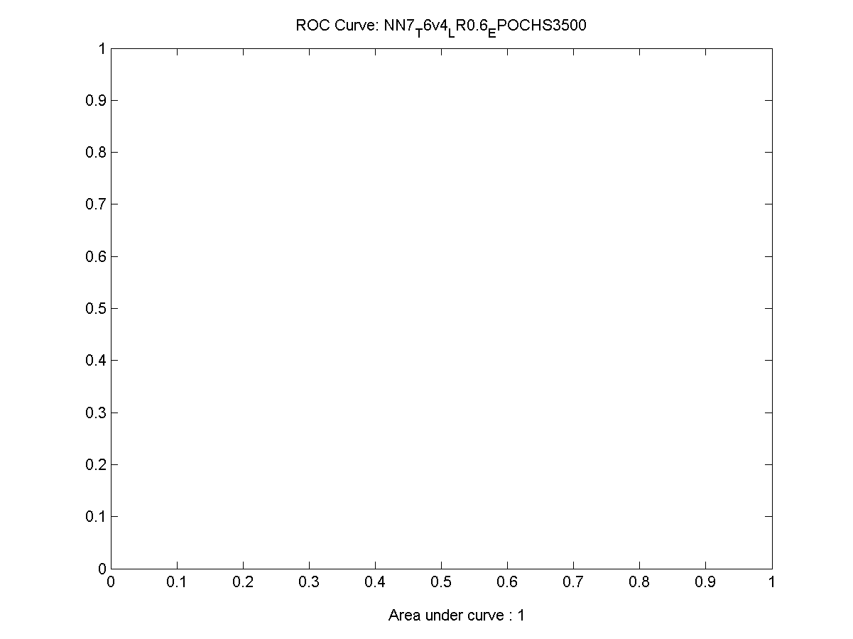
Figure 49 ROC Chart for the best performing network
Figure 49 infers that no misclassification took place for the networks, this was the best performing network with consideration of the area under both ROC curves.
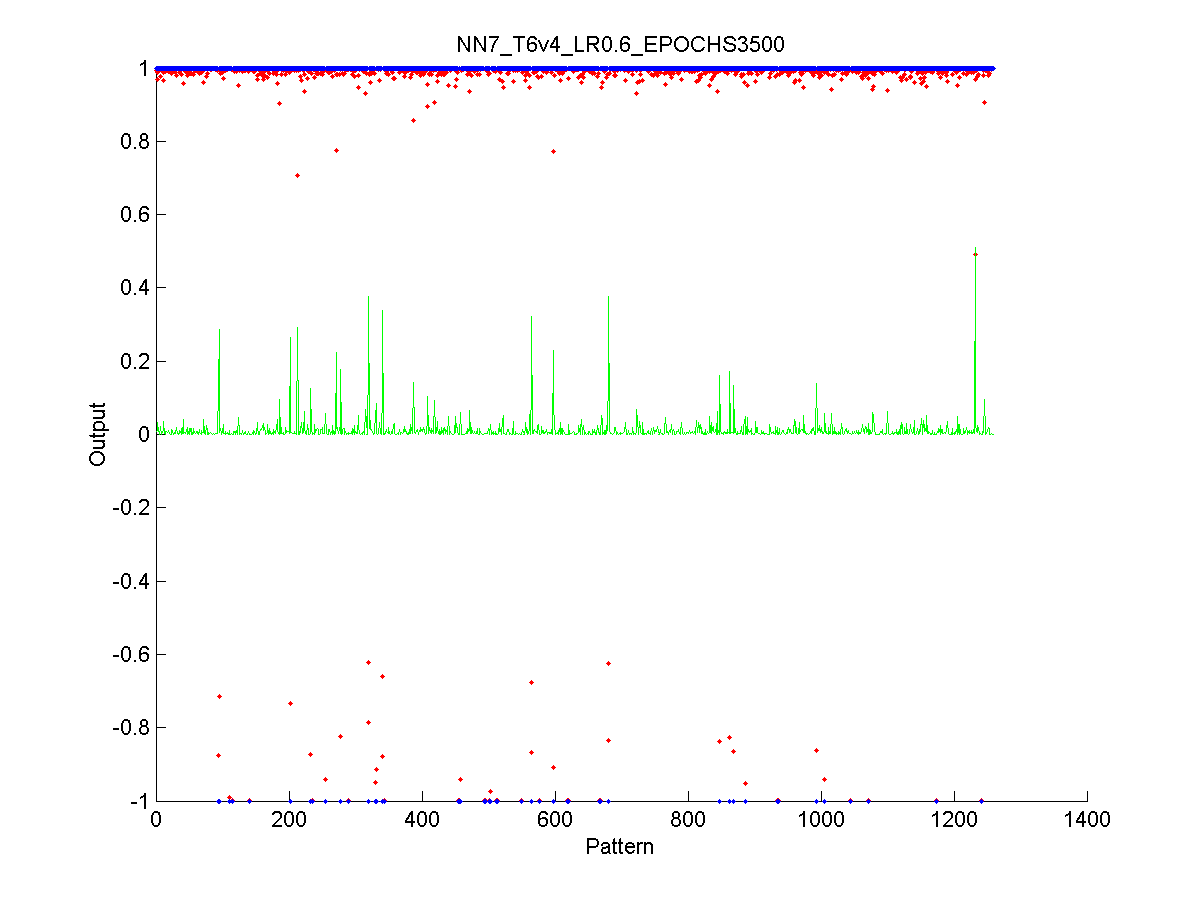
Figure 50 Output from the training data.
It is clear from figure 50 as to why the ROC charts' areas where 1, it can be seen that there is a clear region in which none of the customer accounts can be confused between either of the two classes, with very little error between the desired output and the actual output of the network.
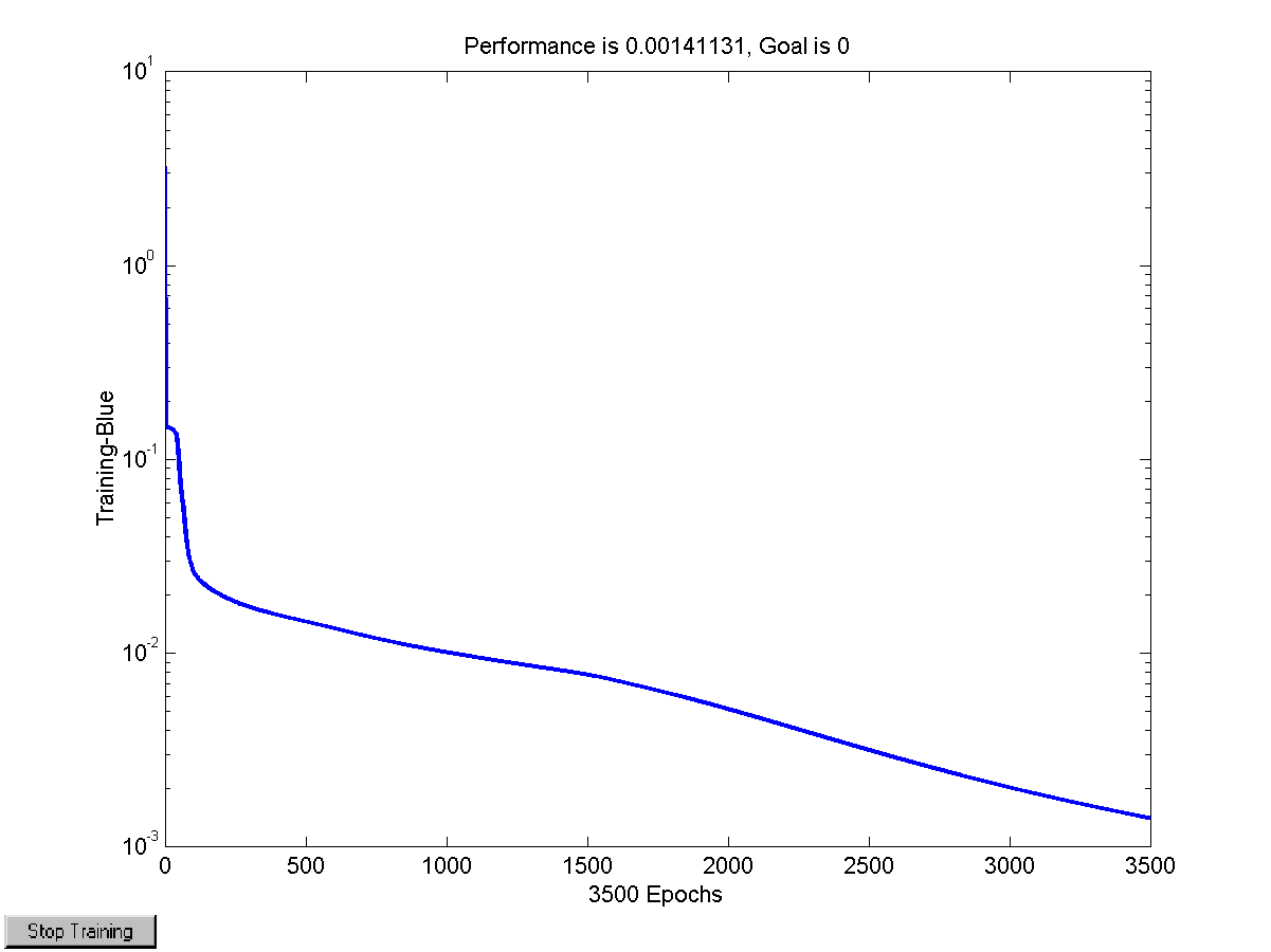
Figure 51 Performance of the final network while training
The overall MSE (Mean squared error) for this network after training is not the smallest of any of the neural networks. This implies that even though less error could have been achieved while training, the result is that the neural networks with a smaller MSE might have been over trained and therefore have become too specific and cannot thoroughly cope with new unseen data. However the training session for this network was very good, after each iteration the network got closer and closer to converging on a solution. The rate of change of the error was extremely steep in the first 100 training sessions, after which the rate at which it trained slowed down but appear constant, indicating that the error was getting reduced steadily after each training session
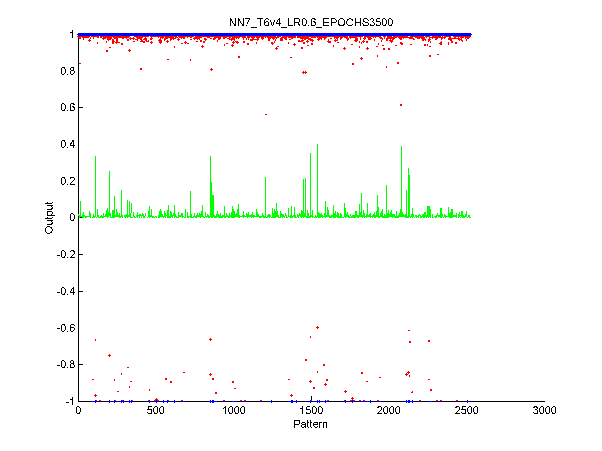
Figure 52 Output from the validation data
Again it is clear from figure 52 as to why the ROC charts' areas where 1, it can be seen that when presented with the validation data there is a clear region in which none of the customer accounts can be confused between either of the two classes. The actual classification of all the clear customers' patterns is very close to the desired output; even the classification of all the fraudulent accounts is very close to the expected output of the network. Both of these cases reinforce the fact that this neural network is the best one available.
10.8.1 The weights from the input layer to the hidden node
The weights that are attached to are shown below, rounded to two decimal places. These would be the weights used if I were to propose this to a company who had real data that was similar to my generated data.
|
|
Inputs weights |
||||||||||||||
|
Link To Hidden Node |
|
1 |
2 |
3 |
4 |
5 |
6 |
7 |
8 |
9 |
10 |
11 |
12 |
13 |
14 |
|
1 |
0.72 |
-0.27 |
0.06 |
0.65 |
0.75 |
0.01 |
-0.18 |
0.36 |
-0.43 |
0.51 |
-0.08 |
-0.46 |
0.19 |
-0.46 |
|
|
2 |
-0.28 |
-0.04 |
0.30 |
-0.13 |
-0.22 |
0.22 |
0.32 |
0.15 |
-0.59 |
-0.82 |
0.61 |
0.37 |
0.60 |
0.28 |
|
|
3 |
-0.52 |
-0.64 |
0.36 |
-0.23 |
0.79 |
-1.47 |
0.61 |
-0.78 |
-0.41 |
0.04 |
0.96 |
-1.25 |
-0.26 |
-0.75 |
|
|
4 |
0.56 |
0.30 |
0.36 |
-0.34 |
0.95 |
-0.05 |
-0.17 |
-0.88 |
-0.33 |
-1.37 |
0.81 |
0.33 |
0.16 |
0.87 |
|
|
5 |
-0.25 |
0.63 |
0.52 |
-1.09 |
-0.24 |
-0.28 |
0.21 |
2.14 |
-0.11 |
1.91 |
-0.19 |
-2.65 |
0.31 |
-0.25 |
|
|
6 |
0.64 |
0.27 |
-0.31 |
-0.58 |
0.45 |
-0.26 |
0.61 |
-0.14 |
0.38 |
-0.27 |
0.34 |
-0.59 |
-0.60 |
-0.37 |
|
|
7 |
0.39 |
-0.43 |
0.58 |
0.39 |
-0.61 |
0.28 |
-0.73 |
-0.32 |
-0.47 |
0.69 |
-0.39 |
-0.14 |
0.11 |
0.00 |
|
10.8.2 The weights to the Output Layer
|
|
Weights from hidden node to output node |
||||||
|
|
1 |
2 |
3 |
4 |
5 |
6 |
7 |
|
Output Node |
0.87 |
0.02 |
2.49 |
1.94 |
-4.00 |
0.28 |
-0.66 |
10.8.3 The Threshold
The reason why this network was chosen over the rest is simply because it was trained well enough to be able to correctly classify 100% of the supplied patterns for both the training and validation data and the totally unseen data.
A threshold value of 0.2 , allows for 100% classification of fraudulent and non-fraudulent data, while giving leeway to allow for a bit of uncertainty when considering if an account is fraud. Because this threshold is near the middle of the output range, all future customer accounts should be correctly classified even if they vary somewhat more than anticipated from the expected customer models.
10.8.4 Proposed Training Regime
Part of the reason why neural networks are good is because they can easily be retrained, every month (or whatever period the telecomm company decides) the phone company could retrain the network with a selection of all the customer data again this would then include the frauds that had been found in the previous month. The retraining would allow new trends to be picked up by the neural network with minimal fuss. As the process of gathering the training data would be the same each time the network needs to be retrained.
If the network needed to be retrained again, extracting from the results the best method to use is normal gradient descent and a learning rate of 0.6; this seemed to give the best trade off between fast convergence on a solution by minimising the time it takes to reach a minima, against the likelihood of the network not training because the learning rate was too high and the gradient could find the minima in the error function.
11. Evaluation
This is an evaluation into the success of the project; the overall aim of the project was to generate a solution that would viable in the telecommunication industry therefore the evaluation will only cover the success of the neural network.
11.1 Does it work?
Broadly speaking the project was in my view a complete success. The top performing networks could classify close to 100% of the input patterns supplied to them, compare this to the performance of Michiaki Taniguchi's 37 neural network which achieved rates of 85% correct detection. However, I am the first to admit that this success might be sullied by the fact that the models created could be conceived to be too simplistic and not truly mimic that of how real customers behave. This was my first ever attempt at a research based software engineering project, which brings several other firsts: I have had to learn about creating models of real-world situations; understand statistics that I have never used before and learn about neural networks.
I can say that the current solution may not work with a telecommunication company because the neural network was trained on data that had to generated using a specially developed tool, but the techniques developed here with a little bit of tweaking and further evaluation can be used to great effect in the telecommunication industry.
The main problem when judging which network performed the best was that too many of the networks that I created performed exceptionally well on both tests. This lead to confusion when considering which network should be the final network.
11.2 Is it Real-time?
The short answer is yes it can operate in real-time. The longer answer is, the network itself can operate in real time, and provide a real-time response once presented with an input. It is the data acquisition, which is the slow part and would eventually bias the classification of whether this project can operate in real-time towards the 'No it is not real time'. Luckily this misclassification can be reduced with the ambiguity relating to what real-time actually means. As defined near the beginning of this project, soft real-time is the solution that is most appealing to this type of project.
The overall speed of the neural network is extremely quick; the computer used to test the networks can classify some 5000 two-week customer profiles in roughly 3 seconds.
11.3 Which Training Method was Most Appropriate
During the analysis of the results, I found that simple gradient descent was more effective than gradient descent with moment. The reason being was that the results indicated that a very large proportion of the networks that did not train correctly used gradient descent with momentum as their training function. This is contrary to my initial understanding and will need more testing by adjusting the momentum coefficient.
11.4 Other Points About the Neural Network
One additional item I noticed when developing the neural networks was that as the number of hidden nodes increased, the number of unsuccessfully trained networks increased. Considering a network that had a ROC area of less than 0.6 meant it could not classify any of the fraudulent customer call patterns and these networks were then disregarded. I would have expected that more training would be needed every time extra hidden nodes were added to the network and performance might therefore be degraded if they were not trained anymore (which they were not), however the aftermath of this results suggests the reason why they did not train was because the random numbers assigned to each weight before training starts did not initialise properly, or were somehow insufficient. I am not too sure why this happened, perhaps and further study is required to find the root cause to this problem.
11.5 The CDR Generation Tool
The CDR tool was a success for this project, it allowed me to generate millions of Call details for thousands of customer which without I would not have been able to test if a neural network was a worthwhile solution.
The CDR Tool could generate over 1000 customer details in less than 20 minutes with each customer having hundreds of calls made.
The models were not the most accurate, but could be developed further if more research into customer calling patterns takes place. More accurate models will produce a neural network that can more accurately model customer calling patterns.
12. Project Management
The project required a great deal of time management; although I am fairly happy with the way in which I worked and the manner in which I followed the time plan I gave initially and the amended time plan that was handed in at Christmas. Several problems arose including the timing of other coursework's for other courses and the unexpected duration of the analysis of the results. What follows are the three time plans
- The predicted time plan at the start of the project
- The amended time plan at Christmas
- The final time plan of all the work that has been carried.
As can be seen, I have managed to stick fairly well to the time plan, however I ended up increasing the time of development and reducing the time for testing. The time spent generating the CDR and analysing the call data was also extended and shifted since at the start of the project I did not consider that the development stage and the call generation stage where dependant on each other and really should have been specified as the same task.
To keep the continuity of the project, the time plans are provided in the appendix
13. Conclusion
This project has proven to an extent that fraud detection using call pattern analysis with neural networks can work. It has however been limited by the lack of real world data and even though a competent call generation tool can be created, I feel that it will never be a substitute for using real data for a real telecommunications company which will provide real results from the neural network that will prove how effective a neural network can be at detecting fraud. Especially as the methods which fraudsters uses is constantly evolving, a method of detection which can evolve with their changing trends (both via generalisation and retraining) will no doubt be a useful tool in any fraud analysts belt.
This project further shows that a neural network is not the only solution to detecting fraud, firstly a company wide fraud strategy needs to be in place with a company wide sharing of resources. For instance, neural networks may not be the optimal method of detecting when people are using false information; in addition, what is the point of having a fraudulent call detection system in place when someone is acting fraudulently on your network if your subscription process keeps allowing the same fraudster back on to the network.
13.1 How I handled the project
This section is a critical appraisal into where I feel the some of the flaws in this project where located. I am doing this because it will allow me to identify in the future where potential problems may arise. The successes of the project will be briefly discussed in the next section (13.2).
From starting with the training in fraud detection in the financial market which I already possessed, I have had to transfer the knowledge onto a totally different domain of fraud detection. This meant learning more about general fraud, the telecommunication industry and specifically more about fraud in the telecommunication industry.
I feel that the research stage of this project went well; although I found it difficult to present only information that was pertinent to the project with out going off on too much of a tangent.
The distinctions between the calls either being High Risk or Low Risk was a piece of the system that I liked as it allowed me to vastly reduce the number of inputs to the neural network; this would have had the effect of allowing the neural network to train faster and generalise better. I would have liked to ran some principle component analysis on the data through MATLAB as this might have been able to highlight more areas where I could have combined data inputs and still got the same meaning from the data, unfortunately time was not on my side for this so I was never able to include it in the project as would have had to analyse both the performance methods of combing the data and compare and contrast their benefits.
I feel that the need to develop a call generation tool essentially detracted the focus of the neural network away from this project, as I feel this made the project the size of two projects and therefore some of the information that I would have liked to put in the project (such as the mathematical functioning of the neural networks) had to be left out so to keep the length of this project within reasonable limits. Saying that I feel even though I have had to shorten this project, the report still seems to be a bit too long. Neither of the project design stages could be documented in this report completely as there would simply be too much information for the reader to process so I had to simply opt for a verbose description of the important algorithms pertinent to the project. Low-resolution flow charts were provided (charts that document the whole system operation not individual functions) to give insight as to how all the separate parts of the project should fit together.
So many neural networks were created, many of them with very similar performance, I had to think up a performance metric that would allow me to classify the results in such a manner that I could give justification to my final choice of network. I am pleased with the results of this performance metric, although I am not sure if it is an original piece of work (as I have found no mention of it anywhere) or if it stands up to rigorous statistical proof in to the worthiness of the method. I am sure that it won't and if I had more time, I would have liked to find better ways to measure relative performance of the neural networks. Therefore I feel that this is another area where I feel that my learning's and implementation lacked clarity and drive.
The neural networks were generated twice; I have already mentioned that I thought the models were possibly slightly weak (section 11.1); this was the second time that I created a set of models for the data. The first time there were only seven models and the neural networks had no trouble at all at classifying them (They are they are the first seven models shown in the appendix ). The second time I created several more models and changed the CDR Generator; the neural networks had a harder time classifying the results correctly, this had the effect of bringing the neural networks performance more inline with that of a neural network which might be deployed in a real world situation.
A revision of the code used to create the customer call records occurred during the lifetime of the project, this was too add attributes into the call records to allow them to mimic customers more effectively. Even though this was in the middle of the development cycle, due to the framework I already had in place it did not affect the overall timing of the project but did mean that the development time was extend.
The revision in the code took the form of:
- Adding in the probability of calls happening on a given day (This was left out until I realised calls in real life are not in spread evenly over the week rather certain days are more likely to have more calls than other days)
- Including the available phone numbers that a customer can ring (although not used by the neural networks) added extra realism to the data generated.
The time plans were altered and can be seen in the appendix 16.6.3. I don’t think that this slight mishap could have been avoided, and like many software engineering projects using the linear sequential model you have to go back a few stages to fix the problem (in this case it was a simple case to reanalyse the inputs to the neural network and an easy fix for the design for the CDR tool).
13.2 What have I learnt?
I have learnt the basic fundamentals of neural networks, obviously I have only scratched the surface of neural network theory and design, but I feel that what knowledge I have gained is the first step on a long road to understanding neural networks and their applications not only in the fraud detection industry but elsewhere as well.
I have also learnt that creating neural networks is not simply a process of training the network and then putting it to use. Rather a proper plan of how you intend to test a possible range of neural networks needs to be put in place before testing even begins. This includes sufficient analysis of the results which the neural networks produce so that the network we choose as the one to be used in a proposed system is the most efficient one which we can develop.
I have learnt about prototyping systems such as MATLAB and how they can be used to model potentially commercially viable systems. From starting with absolutely zero experience of MATLAB, I feel that I can quite confidently use this to model any future systems that I come to develop in my career.
This was a good exercise and first step into model generation. Models are useful for predicting if a certain theory can be proven to be correct (like this project), you can test the theory against the models before moving on to test against real world data. This is also a draw back because a model of a population can never have the same significance as real data and therefore it holds that if it works for a model it may not work for the real thing.
I have shown the Microsoft Access can be used to great effect when considering customer model generation, granted some of the model may have been overly simplistic but if it were to be used in a live environment then a higher degree of refinement would take place. To some extent I found the MS Access would start to play up when more than 300MB of data was being stored in the database, therefore if I could I would like to use MS Access as the front end tool to a more robust RDBMS.
A model generator such as the one developed for this project would be useful for start up communications companies. New companies are more prone to fraud, as fraudsters may (sometimes correctly) assume that new companies do not have the resources of a "more established" company to detect fraud and also do not know what fraudulent activity of customers may look like.
Overall, this project has taught me more about time management and the software engineering process than any of the other projects or coursework's though my life in university since the workload required by this project has been astoundingly large.
The next stage is to take the techniques used in the creation of the network, and apply it to real data from the telecommunication industry, only then can I state fully whether a neural network solution to fraud detection is viable.
14. Further Work
I have identified several key areas, in which this project can be extended if required. Some of these features are extensions that I would have liked to put in if I had the time, while others are extensions to the project that may enable this project to be used as the basis of further work.
Firstly using data that can be gathered from real customer data from real telecom companies would be the first expansion on this work. This would enable myself, or anyone following on from this project to finally prove that neural networks are suitable for fraud detection.
A system that can monitor change in behaviour as well as what the current implementation achieves would be an extremely useful tool. This is because fraudsters may try to hide their fraudulent acts by impersonating a real customer for their first few billing periods, then once their accounts have reached a certain maturity level, they would activate their major fraud operation. This system should then be able to alter the fraud management team to suspicious call activity which is out of the norm for the customer.
To account for behaviour change occurring like the above; an enhancement would require the alteration of the CDR generator time. I have had several thoughts in ways this can be implemented based on the following two ideas.
- Use the current neural network, but have the data access tools aggregate the data over times ranging from two months, to two weeks. This is essentially reducing the granularity of the analysis, if there is substantial change towards fraud in the smaller time capsules in relation to the others and then it may be that someone has started a fraud operation.
- Use the same principle as mentioned previously, but this time if we are looking at two time periods in sequential order, make the input to network, which is analysing the second time period include the fraud score that the previous network gave, thus if the weighting to fraud is higher on a previous data segment, have it effect the next run through the neural network take this into account.
These are just theories that would need to be fleshed further out before embarking on a research project.
The system could have also been extended by including some method of establishing if the customer is constantly calling hotspots (known high risk phone numbers). For instance, calling particular foreign PRS lines would be considered suspicious and is not currently handled by either the CDR generation tool or the neural network model.
Establishing the time between telephone calls would also be a good enhancement, as this could then be used to establish to a higher degree of certainty if a customer is using an automated dialling tool.
Also knowing how long a customer has been with the company and using that as an input to the neural network would also be a good indicator of fraud. It is likely that a customer of five years is not going to be fraudulent, so when analysing their call patterns you would allow for some leeway if the customers recent call pattern has changed or exhibited fraudulent patterns recently. However a customer could be about to move house, use as much of the phone as they can, and then never pay the bill (which is fraud). Obviously further research into this is required.
Furthermore, this project can be considered the starting point for a full blown FMS, the techniques used in this project could be implemented in a system that would automatically generate neural networks based on call information supplied, train on this information and then be used in a live environment. The FMS could then be linked to other system inside the business such as Billing and Subscription. All these departments could then benefit from the use of such a tool.
Although detection of fraud in fixed line communication has been the focus of this project, other important areas of the telecommunication industry also need fraud detection, in particular IP fraud where hackers know how to obtain free Internet based services from the telephone company. Using similar pattern recognition methods as used in this project I think the project could be extended to find when a customers Internet service usage is suspicious.
15. References
- Roger S Pressman : Software Engineering A Practitioners Approach, Chapter 6 Pages 148 – 151
- Computer Networks, Third Edition : Andrew S. Tanenbaum, GSM pages 266-275
- Telestial – A SIM History: http://www.telestial.com/prepaid_more.htm
- National Statistics : "Households with home telephones 1971-2000: Social Trends 31", www.nationalstatistics.gov.uk
- National Statistics : "Home Net Access Up: 11.4 million UK homes now online" www.nationalstatistics.gov.uk
- Computer Networks, Third Edition : Andrew S. Tanenbaum, Circuit Switching pages 130-134
- National leased lines in the UK Summary of Oftel’s investigation : Annex A: BT’s prices for leased lines http://www.oftel.gov.uk/publications/1999/competition/lls0199.htm#Chapter%206
- National leased lines in the UK Summary of Oftel’s investigation : Chapter 6 Competition in the provision of leased lines in the UK http://www.oftel.gov.uk/publications/1999/competition/lls0199.htm#Chapter%206
- UMTS Forum : What Is UMTS
http://www.umts-forum.org/servlet/dycon/ztumts/umts/Live/en/umts/What+is+UMTS_index
- 3G Breakeven Doubtful : http://www.3g.co.uk/PR/October2002/4186.htm
- INTERCONNECTION AND INTEROPERABILITY : A framework for competing networks http://www.oftel.gov.uk/publications/1995_98/interopa.htm#CHAPTER%202
- Victims of Consumer and Investment Fraud : http://www.crimes-of-persuasion.com/Victims/victims.htm
- Telecommunications (Fraud) Act 1997 : http://www.hmso.gov.uk/acts/acts1997/1997004.htm
- Combating Against Telecom Fraud: Introduction http://www.mmtelcom.com/webdex/fraud_prev.html
- Combating Against Telecom Fraud: Losses due to fraud at the world telecom market
http://www.mmtelcom.com/webdex/fraud_prev.html
- The Communications Revenue Assurance and Fraud Management Handbook Yearbook 1999-2000:
- BT Plc: PRELIMINARY RESULTS - YEAR TO 31 MARCH 2002 http://www.btplc.com/mediacentre/Archivenewsreleases/2002/Xq402release.htm
- A Management Guide to the Prevention of Telephone Fraud in the UK 1998 : Siemens Communication Unlimited
- Experiences in Mobile Phone Fraud: Jukka Hynninen; Chapter GSM cloning
http://www.niksula.cs.hut.fi/~jthynnin/mobfra.html
- The Communications Revenue Assurance and Fraud Management Handbook Yearbook 2000-2001: Billing Integrity
- The Communications Revenue Assurance and Fraud Management Handbook Yearbook 1997-1998: Fraud Types
- The Communications Revenue Assurance and Fraud Management Handbook Yearbook 2000-20001: The Enemy within
- Classifying Fraud - The 4 M's: http://mujweb.atlas.cz/Obchod/ordema/fraud.htm
- The Fraud Risk Management Cycle (FRMC) : Fraud Risk Solutions http://www.fraudrisk.com.au/frmc/
- The Communications Revenue Assurance and Fraud Management Handbook Yearbook 1999-2000
- Fighting Telecom Fraud: Cerebrus Solutions Limited; Slide Loss by value
- Definition of Fraud Detection Concepts: ADVANCED SECURITY FOR PERSONAL COMMUNICATIONS TECHNOLOGIES http://www.esat.kuleuven.ac.be/cosic/aspect/
- Fraud Detection In Communications Networks Using Neural and Probabilistic Methods: Michiaki Taniguchi et al; Section 2.3 Bayesian networks
- Applications of Neural Networks to Telecommunication Systems: Fraudulent Use of Cellular Phone Detection : RJ Frank et al
- Discovery of Fraud Rules for Telecommunications - Challenges and Solutions: Saharon Rosset et al
- FRAUD CONTROL: http://www.ctl.com/News/CTLinNEWS/article4.htmd
- Detecting Fraud in the Real World: Michael H. Cahill Chapter 2 Fraud Detection Based on Thresholding
- Bayesian Belief Nets : http://www.cs.ualberta.ca/~greiner/bn.html
- Bayesian Belief and Decision Networks: http://www.norsys.com/belief.html
- Bayesian Belief Network: http://www.murrayc.com/learning/AI/bbn.shtml
- Fraud Detection In Communications Networks Using Neural and Probabilistic Methods: Michiaki Taniguchi et al; Section 2.3 Bayesian networks
- Fraud Detection In Communications Networks Using Neural and Probabilistic Methods: Michiaki Taniguchi et al; Section 2.1 Neural networks with supervised learning
- An Introduction to Neural Networks: Kevin Gurney; Chapter 1 pages 1-6
- Pattern Recognition Using Neural Networks; Theory and Algorithms for Engineers and Scientists: Carl G. Loony; Chapter 3 MLP as Pattern Recognisers
- An Introduction to Neural Networks: Kevin Gurney; Chapter 4 & 6 pages 46, 74
- An Introduction to Neural Networks: Kevin Gurney; Chapter 1 & 6 pages 4, 80
- Neural Network : http://hugroup.cems.umn.edu/Research/plant/neural.htm
- What is a Neural Net ?: http://www.cormactech.com/neunet/whatis.html
- Real-time Systems Lecture Notes : Qi Shi
- Software Engineering A Practitioners Approach : Roger S. Pressman; Chapter 2 pages 26-29
- SQL FAQ, SQL Standard : http://epoch.cs.berkeley.edu:8000/sequoia/dba/montage/FAQ/SQL.html
- Understanding ODBC and OLE: http://msdn.microsoft.com
- MySQL General Information: http://www.mysql.com/documentation/mysql/bychapter/manual_Introduction.html
- PostgreSQL: http://advocacy.postgresql.org/
- Oracle 9i RDMBS : http://www.oracle.com/ip/deploy/database/oracle9i/
- Microsoft Access RDBMS: http://www.microsoft.com/office/access/evaluation/guide.asp
- The Gaussian Distribution : http://www.graphpad.com/instatman/TheGaussiandistributionandtestingfornormality.htm
- Eric W. Weisstein's Math World; The Gaussian Distribution : http://mathworld.wolfram.com/GaussianDistribution.html
- Perl Cookbook : Tom Christiansen & Nathan Torkington; Chapter 2.10 Generating Biased Random Numbers page 54-55
- Perl Cookbook : Tom Christiansen & Nathan Torkington; Chapter 2.10 Generating Biased Random Numbers page 55-56
- An Introduction to Neural Networks: Kevin Gurney; Chapter 1 pages 1-6
- An Introduction to Neural Networks: Kevin Gurney; Chapter 2.2 Artificial neurons: The TLU pages 13-17
- An Introduction to Neural Networks: Kevin Gurney; Chapter 2.4 Non-binary signal communication pages 17-20
- Fundamentals of Neural Networks; Architecture, Algorithms and Applications : Laurene Fausett; Chapter 1.4.2 pages 17-19
- What if it's not linear? (nets): Alun Jones, Institute of Biological Sciences, University of Wales http://users.aber.ac.uk/auj/talk/depttalk97/nets.html
- An Introduction to Neural Networks: Kevin Gurney; Chapter 6 The Multilayer Perceptron and Back propagation pages 65-91
- recurrent link
- Pattern Recognition Using Neural Networks; Theory and Algorithms for Engineers and Scientists: Carl G. Loony; Chapter 9.5 General Principles for Neural Engineering
- Fundamentals of Neural Networks; Architecture, Algorithms and Applications : Laurene Fausett; Chapter 6 Back propagation Neural Net pages 289-290
- An Introduction to Neural Networks: Kevin Gurney; Chapter 6.1 Training rules for multilayer nets pages 65-67
- An Introduction to Neural Networks: Kevin Gurney; Chapter 6.5 Speeding up the learning: the momentum term page 71
- An Introduction to Neural Networks: Kevin Gurney; Chapter 6.3 Local versus global minimums page 69-70
- An Introduction to Neural Networks: Kevin Gurney; Chapter 6.2 The back propagation algorithm
- Pattern Recognition Using Neural Networks; Theory and Algorithms for Engineers and Scientists: Carl G. Loony; Chapter 9.8 The Processes of Training and Validation
- An Introduction to Neural Networks: Kevin Gurney; Chapter 6.7 The action of a well trained net; pages 73-76
- An Introduction to Neural Networks: Kevin Gurney; Chapter 6.9 Generalisation and overtraining; pages 80-83
- Pattern Recognition Using Neural Networks; Theory and Algorithms for Engineers and Scientists: Carl G. Loony; Chapter 10.6 Data Engineering ; pages 352-358
- MATLAB Neural Network Toolbox : Pre-processing and Post-processing; Chapter 5-61 page 189.
- Receiver Operating Characteristic Curves : SAS Institute; http://jeff-lab.queensu.ca/stat/sas/sasman/sashtml/stat/chap39/sect33.htm
- Receiver Operating Characteristic (ROC) curves: http://www.cs.washington.edu/homes/djp3/Compbio/quals/paper/node15.html
- Threshold-independent measures: http://obelia.jde.aca.mmu.ac.uk/multivar/roc.htm
16. Appendices
16.1 Bibliography
- Experiences in Mobile Phone Fraud : Jukka Hynninen http://www.niksula.cs.hut.fi/~jthynnin/mobfra.html
This paper provides information concerning in particular fraud with mobile phones.
- Principles of Data Mining : Hand, Manilla & Smyth;
Discusses some of the considerations when trying to extract data used for statistical processing from a database
- A Basic Course in Statistics : Clarke & Cooke
This book supplied with information and algorithm concerning statistical properties such probability, standard deviations and normal distributions
- Introducing Statistics : Upton & Cook
This book supplied with information and algorithm concerning statistical properties such probability, standard deviations and normal distributions
- An Introduction to Neural Network: Kevin Gurney
This book was my main reference to neural networks, I recommend it if you are unfamiliar with neural networks and would like extra information about neural networks.
- Pattern Recognition Using Neural Network; Theory Algorithms for Engineers and Scientists: Carl G. Looney
This book was one of my secondary references to neural networks which I used when I was unsure about a particular item concerning neural networks or my main reference was not clear enough.
- Fundamentals of Neural Networks; Architecture, algorithms and applications: Laurene Fausett
This book was the second of my secondary references to neural networks which I used when I was unsure about a particular item concerning neural networks or my main reference was not clear enough.
- Applications of Neural Network to Telecommunication Systems: RJ Frank et al.
Contains ideas about methods to detect fraud using neural networks as well as some other uses of neural networks in the telecom industry
- Activity monitoring: Noticing Interesting Changes in Behaviour: Tom Fawcett & Foster Provost
Contains information I would use if I were to extend this project in to monitoring for changes in behaviour.
- Detecting Fraud in the Real World: Michael H. Cahill et all.
Contains a lot of information about different fraud detection methods in relation to credit cards and telecoms and fraud in general
16.2 Program Listing
The program listings have not been supplied in this report so that the size of the report is kept to a minimum, rather they have been included on a CD stored in the appendices.
There are two sections to the program listing. The MATLAB section and the Microsoft Access 2000 section:
- The MATLAB section contains the workspaces that were used throughout the development and also the code that was created for the automated neural network creation and testing tools. Each of the MATLAB files is fully commented and are exact digital copies of what would normally be present in this section.
A brief overview about what each of the functions achieves is included in this section.
- The Microsoft Access 2000 section contains the MDB that is the actually application that was created to make all of the customer calls. The code listing on its own would be useless without the necessary information about the windows forms used in this project. However, the documentation tool that Microsoft Access provides, outputs more information than is needed and also even with the basic information which would provide a overview of the system the output would run into approximately 30 pages.
Other than just the code listings are the queries that were used through out the project to aggregate the data. Many of these queries are extremely long and are also nested to such an extent that a simple output of the code will give no indication as to what is happening in the system.
Instead Screen shots have been provided with an a explanation to the parameters used in model creation.
Overall the project would be extended by more than 60 pages none of which would provide any significant advantage over providing the code listings on a CD.
16.2.1 MATLAB Overview
This section details the code and the performance information related to the MATLAB section of this project.
16.2.1.1 How to read the performance information off the CD
Each of the performance graphs are stored on the CD under the directory Matlab. To make it easier to read the graphs each network that has a different number of hidden nodes stores the graphs in the directory nn x, where x signifies the number of hidden nodes.
Each neural network that was created has a name. This name is used in each of the file names; the type of graph created is appended to the end of the file name.
The name contains information about the network parameters.
NN5_T1v1_LR0.1_EPOCHS1000
The network has 5 hidden neurons (NN5), was trained on gradient descent (No training qualifier), some versioning information (T1) training data combination 1 (v1), the learning rate 0.1 was used (LR0.1) and the number of training sessions was 1000 (EPOCHS1000)
NN5MOMENTUM_T3v1_LR0.3_EPOCHS1000
Networks trained using gradient descent with momentum can be seen because they have the classifier MOMENTUM in.
Each network that has been created has at least 4 graphs:
- Normal Performance Graph (Takes the form of the network name.png )
- ROC chart for the first performance test ( network name)_ROC.png )
- Output of network after test stage ( network name-Testoutput.png )
- Output of network after validation ( network name-Validationoutput.png )
16.2.1.2 Function Descriptions
A brief description of the functions that are used to help me generate and test all the neural networks is provided below.
|
Function |
Description |
|
AreaROC |
Returns the area, sensitivity and the 1- specificity of the neural network. The output is NOT stored to disk. |
|
countPercentageGroup |
Counts the number of neural networks whose performance is 100 - x% smaller than the largest error (difference between neural networks). For instance, if we want to find all the networks who have only 10% difference in the area in relation to the largest error. There error performance must be 90% smaller than the largest error. |
|
getData |
Retrieves all the data needed for the inputs of the neural networks. All data aggregation is performed in the MS Access queries and not in this query. |
|
getDistance |
Gets the difference between the two areas of the ROC charts for each neural network |
|
getOutputData |
Get the desired outputs from the database. These are the outputs that the network compares itself against when training the neural network. |
|
makeNNMom |
Crates, trains and outputs all the performance information concerning the neural networks to be trained using gradient descent with moment. |
|
makeNNs.m |
Crates, trains and outputs all the performance information concerning the neural networks to be trained using gradient descent. |
|
normaliseData |
Get the parameters so that the data can be normalised so that the inputs fall in the range of -1 and 1. |
|
plotErrors |
Creates the graphs used to visualise how the neural network output has compared to the expected output. Stores the information on disk. |
|
retest |
Tests all the neural networks on the new data which the networks have never seen before. Establishes the ROC chart for the new simulation and stores information about the area under the ROC chart and the difference between ROC chart areas for the different network simulations. |
|
ROC |
Used to store and generate information about the ROC chart for each neural network (such as all the data points and the area) and also outputs the graph to disk. |
|
seperateData |
Splits the data into 4 separate sets of data so that the neural network is trained on a "random" sample of data. |
|
setupConnection.m |
Creates the ODBC connection that is used in every function that pulls data from the database. |
16.2.2 MS Access Overview
The code itself if documented inside MS Access, however the queries that are used are not, and they require brief explanation in order to understand what they are meant for. The SQL is not provided as this can be seen when entering the design view of any of the queries.
|
Query Name |
Description |
|
Free |
Append list of valid free phone std codes in to the database |
|
Intl |
Append list of valid Intl std codes in to the database |
|
Local |
Append list of valid Local std codes in to the database |
|
Mobile |
Append list of valid Mobile std codes in to the database |
|
National |
Append list of valid National std codes in to the database |
|
PRS |
Append list of valid PRS std codes in to the database |
|
qryAllOutputs4Weeks |
Gathers all the outputs that is required for the neural network to train from. |
|
qryCallInfo4Weeks |
Gathers information about the number of calls made per customer over a bi-monthly period. |
|
qryCallSummary4Weeksv2 |
This is the amalgamation of all the other queries. It is used by the neural network software to provide aggregated data to the network for training. |
|
qryCodeCounts |
Used when creating a customers valid dialling code proportions. |
|
qryGetLocalCodes |
Get all the local std codes, so that valid phone numbers can be generated |
|
qryHighRisk-CallSummary4Weeks2 |
Gather all data about high risk calls for each customers bi monthly period |
|
qryLowRisk-CallSummary4Weeks2 |
Gather all data about low risk calls for each customers bi monthly period |
|
qryModels |
Used on the main form to store information about all models that need to be created |
|
qryPeriodIncomming-4Weeks |
Get all information about all incoming calls for a customer |
|
qryTimeData |
Get the data required for the form about when calls can be made. |
|
qryTimeData |
Get the data required for the chart about when calls can be made |
|
qryTimePlans |
Get a list of all the available time plans for a model. |
16.3 CDR Generation Tool Screen Shots
Screen shots are provided to show the work that has been done on the CDR Tool, while also showing what some of the non-obvious parameters are for.
The Source code for any of the forms can be viewed by clicking on the form icon in MSAccess and then going to the "View" menu and then selecting "Code". Alternately the code has been included in a plain text file on the CD.
16.3.1 Screen 1
Information concerning the number of calls everyone in the model will make.
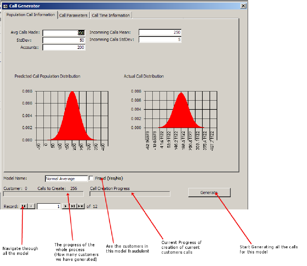
16.3.2 Screen 2
Information concerning durations for each type of call the population and each customer will have in the model.
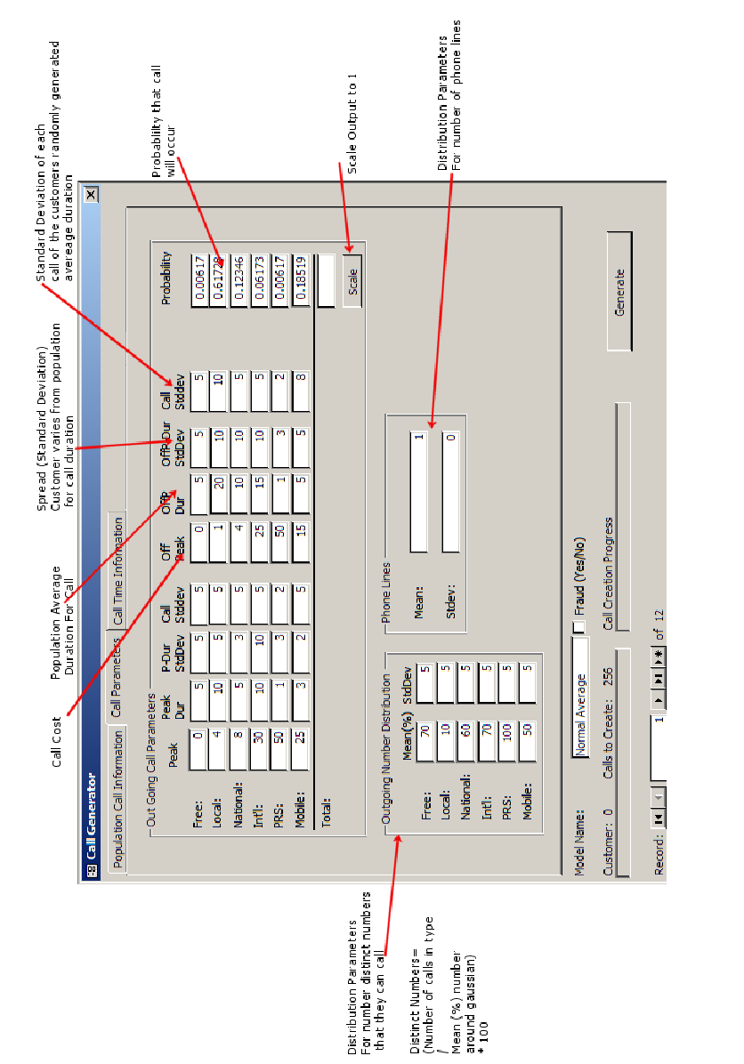
16.3.3 Screen 3
Information pertaining to the times when calls can occur for a given model

16.4 Testing Plan
16.4.1 CDR Tool
The following set of checks is to establish if the random number generators function correctly. Because of the way in which random numbers are generated, we can never get an accurate prediction as to how they will be distributed in a population. Therefore some tolerance has been allowed to judge whether they pass. It must also be noted that the more tests we do the closer to the actual predicted values the result will be.
All of the test to generate the random numbers were ran through the VBA Output window in Microsoft Access 2000.
|
Test |
Expected Result |
Obtained Result |
|
Generate a 500 random Gaussian distributed numbers with a mean 0 and standard deviation 1 (Assess whether values generated by the polar box-Muller method follow a random distribution) |
STDEV: ~1 MEAN: ~0 +/- 0.5 |
STDEV: 0.985 MEAN: 0.047 PASS |
|
Generate 100 random numbers based on three bias values of A) 50%, B) 25% C) 25% |
50 random number classified as A, 25 as B and 25 as C (10% error) |
A: 52 B: 25 C: 23 PASS |
|
Generate 500 random Gaussian distributed number with mean 20 and standard deviation 5 (Assess whether we can transform the values generated by the polar box-Muller method) |
STDEV: ~5 MEAN: ~20 +/- 0.5 |
STDEV: 0.4.973 MEAN: 20.01 PASS |
Now that the correct functionality of the random number generators has been established, it is time to move on to the testing of the model generators. The following test are performed firstly to see if the models can be generated from the random numbers supplied, but also that the models which have been created follow the pattern that the model specifies.
It must again be noted that all the models are based on random number with properties given as weightings, means and standard deviations. Therefore the results obtained will not match exactly what is expected but will follow some semblance of the attributes defined by the model. Obviously the more models we generate in a group the closer that the distributions will match with the predicted distributions.
All of these test were performed using SQL that was generated specifically to test if the model generator worked correctly.
|
Test |
Expected Result |
Obtained Result |
|
Create 200 customers whose number of calls follow the distribution with an average of 300 calls over the time period with a standard deviation of 50 |
STDEV: ~50 MEAN: ~300
|
STDEV: 46.01 MEAN: 297.1 PASS (The more model created the more in line the results will be) |
|
Create 200 customers whose number of incoming calls follow the distribution an average of 600 calls over the period with a standard deviation of 80 |
STDEV: ~80 MEAN: ~600
|
STDEV: 86.975 MEAN: 598 PASS (The more models created the more in line the results will be) |
|
Create a population of 200 customers whose number call distribution of call types is: Free Rate: 1.5% Local Rate: 61% National Rate: 12% International Rate: 6% PRS Rate: 0.5% Mobile Rate: 19% |
Free Rate: ~1.5% Local Rate: ~61% National Rate: ~12% International Rate: ~6% PRS Rate: ~0.5% Mobile Rate: ~19% |
Free Rate: 1.3% Local Rate: 59.1% National Rate: ~13.1% International Rate: ~5.3% PRS Rate: ~0.3% Mobile Rate: ~20.9% PASS |
|
Create 200 customers whose telephone calls they make have the probability of falling on a given day: Monday: 5% Tuesday: 10% Wednesday: 10% Thursday: 10% Friday: 10% Saturday: 35% Sunday: 20% |
Monday: ~5% Tuesday: ~10% Wednesday: ~10% Thursday: ~10% Friday: ~10% Saturday: ~35% Sunday: ~20% |
Monday: 4% Tuesday: 11% Wednesday: 11% Thursday: 12% Friday: 8% Saturday: 33% Sunday: 21% PASS |
|
Create 200 customers and check the populations average call duration for off peak calls, follows the Gaussian distribution based the following:
Free: MEAN: 3 (minutes) STDDEV: 3 Local: MEAN: 25 (minutes) STDDEV: 10 National: MEAN: 5 (minutes) STDDEV: 2 International: MEAN: 12 (minutes) STDDEV: 5 PRS: MEAN: 2 (minutes) STDDEV: 3 Mobile: MEAN: 5 (minutes) STDDEV: 5 |
Free: MEAN: ~3 (minutes) STDDEV: 3
Local: MEAN: ~25 (minutes) STDDEV: 10
National: MEAN: ~5 (minutes) STDDEV: 2
International: MEAN: ~12 (minutes) STDDEV: 5
PRS: MEAN: ~2 (minutes) STDDEV: 3
Mobile: MEAN: ~5 (minutes) STDDEV: 5 |
Free: MEAN: 3.2 (minutes) STDDEV: 3.5
Local: MEAN: 27.3 (minutes) STDDEV: 8.6
National: MEAN: ~4.01 (minutes) STDDEV: 2.03
International: MEAN: 12.59 (minutes) STDDEV: 5.793
PRS: MEAN: ~1.44 (minutes) STDDEV: 2.32
Mobile: MEAN: 5.2 (minutes) STDDEV: 5.64 PASS |
|
From the 200 customers in the previous test, check the average call duration for the off peak calls types of each customer has a standard deviation of that specified for the Gaussian distribution:
Free Calls Average Standard Deviation: 5 Local Calls Average Standard Deviation: 10 National Calls Average Standard Deviation: 5 International Calls Average Standard Deviation: 5 PRS Calls Average Standard Deviation: 2 Mobile Calls Average Standard Deviation: 8
|
Free Calls Average StDev: ~5 Local Calls Average StDev: ~10 National Calls Average StDev: ~5 International Calls Average StDev: ~5 PRS Calls Average StDev: ~2 Mobile Calls Average StDev: ~8
|
Free Calls Average StDev: 4.371 Local Calls Average StDev: 10.15 National Calls Average StDev: 3.58 International Calls Average StDev: 4.45 PRS Calls Average StDev: 2.19 Mobile Calls Average StDev: 8.31 PASS |
|
Create 200 customer accounts with an average of 20 phone lines (company) with a standard deviation of 3 across the population |
STDEV: ~20 MEAN: ~3
|
STDEV: 22.331 MEAN: 3.586 PASS |
|
Check that for 200 customers that a call is 7 times more likely to happen at 7:30pm than at 7:30am. |
~14% more likely to be an evening call about 7:30pm |
Average number of Calls Made at about 7:30 pm: 2.6 per customer Average number of call made at about 7:30am: 0.36 PASS |
The Final set of tests that were carried on the CDR tool were some simple functionality tests to ensure the logic is correct
16.4.2 Neural Network Tools
Each of the major functions used in the training tool creation has had to be tested sufficiently
|
Function |
Test Description |
Test Result |
|
AreaROC |
Test that for any given network it returns the correct area under the ROC chart |
PASS |
|
countPercentageGroup |
Create a temporary set of that have certain errors in relation to their performance on training of both data sets. 10 networks are given an error of between 10% - 20% ensure they are counted. |
PASS |
|
getData |
Check that 1500 bi-monthly customer accounts are obtained from the database. |
1500 accounts returned |
|
getOutputData |
Check that 1500 bi-monthly customer accounts are obtained from the database. Ensure they align with the inputs already obtained. |
1500 accounts returned PASS |
|
makeNNMom Test 1 |
Create a set of 5 layer networks with learning rates from 0.1 - 0.9 (lr increment of 0.1) and 500 - 1000 epochs (500 epoch increments) Are 18 networks created? |
18 networks created. PASS |
|
makeNNMom Test 2 |
Create a set of 5 and 6 layer networks with learning rates from 0.1 - 0.9 (lr increment of 0.1) and 500 - 1000 epochs (500 epoch increments) Are 36 networks created? |
PASS |
|
makeNNs Test 1 |
Create a set of 6 layer networks with learning rates from 0.1 - 0.9 (lr increment of 0.1) and 500 - 1500 epochs (500 epoch increments) Are 18 networks created? |
PASS |
|
makeNNs Test 2 |
Create a set of 5 and 6 layer networks with learning rates from 0.1 - 0.9 (lr increment of 0.1) and 500 - 1000 epochs (500 epoch increments) Are 36 networks created? |
PASS |
|
plotErrors Test 1 |
Is the graph of errors correct in relation to the output of the network and the expected |
PASS |
|
plotErrors Test 2 |
Is the graph of errors correct in relation to the output of the network and the expected and is the graph stored on disk |
PASS |
|
Retest Test 1 |
For each network presented, is the network re-simulated on the new Data created. |
PASS |
|
Retest Test 2 |
For each network presented, is the network re-simulated on the new Data created and is performance information stored. |
PASS |
|
ROC Test 1 |
Create a data set with 0 misclassified results out of 100. Check to see if the area 1.0 |
PASS |
|
ROC Test 2 |
Create a data set with 20 misclassified results out of 100. Check to see if the area approximately 0.85 |
PASS |
|
seperateData Test 1 |
Run test to establish if data is split ¼ training, ¼ test and ½ validation Check if data is interleaved. |
PASS |
|
seperateData Test 2 |
Run test again to see if the has separated on a different view of the data. |
PASS |
16.5 Model Descriptions
The actual model parameters can be seen by starting up the Microsoft Access Database located on the CD.
However, what is included is a brief description of each of the models used in this project.
|
Model Name |
Model Description |
Number of Accounts |
|
Normal Average |
This customer is classed as an average user, one who will make 25 telephone calls each week; receiving approximately 32 calls a week, this was modelled off my relatives. The majority of their calls being local rate calls, in combination with a some national based calls. The likelihood of International calls is slim, but still occur. The probability that they make a PRS call is even smaller than that of International calls, but still may occur. |
200 |
|
Normal No International |
This customer has the same parameters as the "Normal Average" Customer, however they make no international calls at all. |
200 |
|
FRAUD - CALL SELLING International |
This type of call selling is based around the method (4m's) of making money by selling on calls to International numbers at heavily subsidised rates. Therefore we can assume that each of the calls will take a fairly long time to complete, while the times in which the calls operate can be considered to occur at pretty much anytime of the day and likewise for the day in which they occur (as there are international fraud hotspots all over the world). They are unlikely to call other number groups such as local, national etc. |
6 |
|
FRAUD - PRS |
The first type of PRS fraud is based on the fraud where the perpetrators will use an automated dialling tool to call the PRS numbers. These can normally be identified because certain characteristics occur, such as the call length is nearly always the same duration, with very little deviation. |
12 |
|
FRAUD - PRS 2 |
The second type of PRS fraud occurs when a customer will "hammer" PRS lines, that is they will either call one number or many numbers (normally related to the same owner of the PRS line) with the duration of each of the calls taking an extremely long time. |
10 |
|
Business - Shop |
Consider a small shop such as a sweet shop or hairdressers. They may not make many calls during the day and even fewer during the twilight hours. However, they are more than likely to receive more calls from suppliers or customers. Bearing this in mind, another point to consider is the days in which they will make calls. Many small shops are open on Saturdays, this means that they may close on a Monday. Obviously this affects the times of calls, and the call cost, since if the majority of calls they place, occur on a Saturday then these calls all incur off-peak tariffs. |
100 |
|
Business - Small |
A small business could be expected to roughly make at least twice as many calls as they receive. Their calling times also differ from those such as the general public, in that the majority of calls will be placed in the 9am-5pm range. You would also expect them to make roughly equal local and national calls. Again this all depends on the business type, and would need to be established further. This is the first model to approximate the use of multiple lines. This is due to the fact that a company is likely to make and receive multiple calls at the same time. Additionally no PRS calls are made. |
50 |
|
Business - Medium |
Assumptions based on a medium sized company being approximately four times larger than a company in the "small" class. Additional features have been included, such as the probability that a call is an International call occurs is more prevalent than the same parameter in the "Business – Small" class. |
40 |
|
Business - Large |
A Large company could be considered about nine times larger than a medium sized company with respect to the number of calls it makes and receives. Typical accounts might include industries such as banks. However the call properties, such as average call duration would be roughly comparable to those of a smaller company. Again, this is business specific. |
20 |
|
Home - Internet Access |
Home users can also be said to fit into two categories, those who use the Internet and those who do not. This is a very broad simile. However, I have used it to establish if the neural network could establish the difference between these accounts and those that are used in any type of fraud that involves long call durations. For instance, an Internet user will more than likely make a lot of call that last two hours and may have a re-dialler on the system that would automatically log them back on to the Internet. This could be said to mimic the PRS auto dialler model and also the PRS long call duration model |
200 |
|
Home - Plenty Of International |
There are situations when a home customer would regularly call International numbers. Cases such as a family have emigrated to the UK, while the rest of their family are still living in the country of their origin.
Situations that take into account where the families are from is not included (i.e. the location of where the call is being placed to), for instance there is no distinction of someone calling Australia or Zimbabwe. |
200 |
|
Fraud Home Call Sell PRS Hidden |
This model tries to mimic the "Normal Average" model, but with one distinct difference, they are actually hiding PRS fraud in which they make long duration calls the PRS lines in the evening. |
10 |
16.6 Project Management
16.6.1 Time Plan (Initial)
16.6.2 Time Plan (Interim)
16.6.3 Time Plan (Final)
16.7 Interim Report & Specification